library(rpact)
library(ggplot2)
packageVersion("rpact")
[1] '4.5.0'Planning a clinical trial usually involves more than one sample size calculation. How sensitive is the required sample size to the assumed treatment effect? What happens if the variability is larger than expected? Would an interim analysis reduce the expected number of patients, and how much power could be lost by stopping for futility?
This vignette illustrates how getComparison() and compare() bring these calculations together for design decisions. Start directly from a design with |> compare() for a quick comparison, or start with an empty comparison and add named scenarios as they are calculated, using |> add(). Use fetch() to retrieve scenarios and delete() to remove them. We first plan a fixed design for a two-group blood pressure trial and validate the selected sample size with getPowerMeans(). We then extend the example to a group sequential design with one interim analysis and compare several futility rules.
The clinical assumptions are illustrative planning scenarios. These examples supplement the rpact help pages; they do not replace a study-specific justification of the effect, variability, and stopping rules.
library(rpact)
library(ggplot2)
packageVersion("rpact")[1] '4.5.0'Use an rpact version providing getComparison(), compare(), and their associated methods. The package version used to execute this vignette is shown above.
getComparison() collects existing rpact objects: designs, design characteristics, sample size calculations, power calculations, and simulation results. It does not perform another sample size calculation, vary parameters automatically, or choose a preferred design. First calculate the scenarios of interest, then add the resulting objects to the comparison.
To build a comparison incrementally with named scenarios: create it once with getComparison(), then use |> add() whenever another scenario is ready. This works interactively and in loops, without having to assemble all scenarios in a single constructor call. Give scenarios meaningful, unique names so that they remain easy to identify in tables, plot legends, and subsequent selections.
comp <- getComparison()
length(comp)
[1] 0comp |> add(design1 = getDesignGroupSequential(kMax = 2))Design comparison
1 objects; 2 comparison rows; 19 columns.
Object types
Observed metrics (across objects, stages and situations)
Available operations
comp |> add(design2 = getDesignCharacteristics(
    getDesignGroupSequential(kMax = 3)
))
Design comparison
2 objects; 5 comparison rows; 27 columns.
Object types
Observed metrics (across objects, stages and situations)
Available operations
names(comp)[1] "design1" "design2"length(comp)[1] 2The comparison can contain different supported object types, as here. add() appends objects and modifies comp in place, so no reassignment is needed. Names must be unique; adding an existing name raises an error rather than replacing the scenario.
Retrieve an object with fetch(), either by its exact name or its position:
firstDesign <- comp |> fetch("design1")
identical(firstDesign, comp |> fetch(1))
[1] TRUEselectedObjects <- comp |> fetch(c("design1", "design2"), output = "list")
names(selectedObjects)[1] "design1" "design2"A single selection returns the contained object itself. Use output = "list" when a named list is needed, including when selecting only one object.
Scenarios can also be removed as planning evolves. For example, add an exploratory fixed design, then remove it by name:
comp |> add(exploratory = getDesignFixed())Design comparison
3 objects; 6 comparison rows; 27 columns.
Object types
Observed metrics (across objects, stages and situations)
Available operations
comp |> delete("exploratory")Design comparison
2 objects; 5 comparison rows; 27 columns.
Object types
Observed metrics (across objects, stages and situations)
Available operations
names(comp)[1] "design1" "design2"delete() removes one object per call and also modifies the comparison in place. The original design object is not changed by removing it from the collection.
Names are optional. Inspect names() rather than assuming that a generated plot label is also an object name:
unnamedComp <- getComparison()
unnamedComp |> add(getDesignGroupSequential(kMax = 2))
Design comparison
1 objects; 2 comparison rows; 18 columns.
Object types
Observed metrics (across objects, stages and situations)
Available operations
unnamedComp |> add(getDesignGroupSequential(kMax = 3))Design comparison
2 objects; 5 comparison rows; 18 columns.
Object types
Observed metrics (across objects, stages and situations)
Available operations
names(unnamedComp)NULLunique(as.data.frame(unnamedComp)[, c("objectNumber", "objectType")]) objectNumber objectType
1 1 TrialDesignGroupSequential
3 2 TrialDesignGroupSequentialsecondDesign <- unnamedComp |> fetch(2)
identical(secondDesign, unnamedComp[[2]])[1] TRUEunnamedComp |> delete(1)Design comparison
1 objects; 3 comparison rows; 18 columns.
Object types
Observed metrics (across objects, stages and situations)
Available operations
identical(secondDesign, unnamedComp |> fetch(1))[1] TRUElength(unnamedComp)[1] 1For this fully unnamed comparison, names(unnamedComp) returns NULL: add() does not generate stored names. The exported objectNumber identifies each object by its current position; automatically generated display labels are not names for fetch() or delete(). Use integer indices for unnamed entries. Deleting the first entry shifts the second entry to position 1, so recheck positions after a deletion. Explicit names are preferable when scenarios need stable identifiers.
When you want to compare just a few designs that can be specified immediately, passing them directly to getComparison() is also useful. This compact form creates a populated comparison in a single call:
smallComparison <- getComparison(
    two_stage = getDesignGroupSequential(kMax = 2),
    three_stage = getDesignGroupSequential(kMax = 3)
)
smallComparison |> print()
Design comparison
2 objects; 5 comparison rows; 19 columns.
Object types
Observed metrics (across objects, stages and situations)
Available operations
The same two design settings can also be compared by starting directly from the first design and piping it into compare():
pipedComparison <- getDesignGroupSequential(kMax = 2) |>
    compare(getDesignGroupSequential(kMax = 3))
length(pipedComparison)
[1] 2The first compare(x, y) creates the comparison through getComparison(x, y). Further calls append to that comparison, so a third design fits naturally into the same pipeline:
pipedComparison |>
    compare(getDesignGroupSequential(kMax = 4))
Design comparison
3 objects; 9 comparison rows; 18 columns.
Object types
Observed metrics (across objects, stages and situations)
Available operations
length(pipedComparison)[1] 3When its first argument is already a comparison, compare() calls its $add() method and modifies it in place; no reassignment is needed. These entries are unnamed, so use positions to retrieve them. The pipe form also accepts design characteristics, sample size and power calculations, and simulation results, including mixtures of supported object types.
For a quick sample size comparison, calculate three effect assumptions and pass the result straight to summary() in a single pipeline:
getSampleSizeMeans(alternative = 0.22) |>
    compare(getSampleSizeMeans(alternative = 0.44)) |>
    compare(getSampleSizeMeans(alternative = 0.59)) |>
    summary()
Sample size calculation comparison summary
Comparison of 3 sample size means calculations. The comparison identifies 5 differing parameters and 16 shared parameters or profiles. Shared (examples): Object type, Endpoint, Calculation target, Standard deviation, Normal approximation, Mean ratio, … (all shared captions: showAll = TRUE)
Inputs and design settings
Alternatives - numeric, continuous [3 profiles]
| Parameter | Value |
|---|---|
| Sample size means 1 | 0.22 |
| Sample size means 2 | 0.44 |
| Sample size means 3 | 0.59 |
Results and derived parameters
Critical values (treatment effect scale) - numeric, continuous [3 profiles]
| Parameter | Value |
|---|---|
| Sample size means 1 | 0.1539693 |
| Sample size means 2 | 0.3082939 |
| Sample size means 3 | 0.4138996 |
Number of subjects fixed - numeric, continuous [3 profiles]
| Parameter | Value |
|---|---|
| Sample size means 1 | 650.59405 |
| Sample size means 2 | 164.10993 |
| Sample size means 3 | 92.15175 |
Number of subjects fixed (1) - numeric, continuous [3 profiles]
| Parameter | Value |
|---|---|
| Sample size means 1 | 325.29703 |
| Sample size means 2 | 82.05496 |
| Sample size means 3 | 46.07588 |
Number of subjects fixed (2) - numeric, continuous [3 profiles]
| Parameter | Value |
|---|---|
| Sample size means 1 | 325.29703 |
| Sample size means 2 | 82.05496 |
| Sample size means 3 | 46.07588 |
Legend
Complete display: summary(x, showAll = TRUE). Full data: as.data.frame(x). Exact profiles: summary(x)$parameterInfo.
No intermediate variables or explicit comparison constructor are needed. The summary shows how the required sample size changes across the three effect assumptions while the other planning settings remain the same.
Use |> compare() for a quick comparison starting from an existing planning object, pass named objects directly to getComparison() for a small, self-contained comparison, or start empty and use |> add() when named scenarios are calculated progressively or generated in a loop. All forms create the same kind of comparison object and support fetch(), delete(), and the reporting methods below.
The named comparison comp still contains the two sequential scenarios:
comp |> print()Design comparison
2 objects; 5 comparison rows; 27 columns.
Object types
Observed metrics (across objects, stages and situations)
Available operations
comp |> summary()Design comparison summary
Comparison of 2 trial planning results: group sequential design, group sequential design characteristics. The comparison identifies 15 differing parameters and 8 shared parameters or profiles. Shared (examples): Endpoint, Calculation target, Type of design, Significance level, Type II error rate, Binding futility, … (all shared captions: showAll = TRUE)
Object types and scope
Object type - character, factor [2 profiles]
| Parameter | Value |
|---|---|
| design1 | TrialDesignGroupSequential |
| design2 | TrialDesignCharacteristics |
Inputs and design settings
Maximum number of stages - integer, factor [2 profiles]
| Parameter | Value |
|---|---|
| design1 | 2 |
| design2 | 3 |
Information rates - numeric, continuous [2 profiles]
| Parameter | Stage 1 | Stage 2 | Stage 3 |
|---|---|---|---|
| design1 | 0.5000000 | 1.0000000 | |
| design2 | 0.3333333 | 0.6666667 | 1.0000000 |
Futility bounds (non-binding) - numeric, continuous [2 profiles]
| Parameter | Value | Stage 1 | Stage 2 | Stage 3 |
|---|---|---|---|---|
| design1 | -Inf | |||
| design2 | -Inf | -Inf | NA |
Results and derived parameters
Cumulative alpha spending - numeric, continuous [2 profiles]
| Parameter | Stage 1 | Stage 2 | Stage 3 |
|---|---|---|---|
| design1 | 0.0025828932 | 0.0249999900 | |
| design2 | 0.0002591737 | 0.0071600594 | 0.0249999900 |
Critical values - numeric, continuous [2 profiles]
| Parameter | Stage 1 | Stage 2 | Stage 3 |
|---|---|---|---|
| design1 | 2.796510 | 1.977431 | |
| design2 | 3.471091 | 2.454432 | 2.004036 |
Stage levels (one-sided) - numeric, continuous [2 profiles]
| Parameter | Stage 1 | Stage 2 | Stage 3 |
|---|---|---|---|
| design1 | 0.0025828932 | 0.0239964687 | |
| design2 | 0.0002591737 | 0.0070553616 | 0.0225331246 |
Inflation factor - numeric, continuous [2 profiles]
| Parameter | Value |
|---|---|
| design1 | NA |
| design2 | 1.017406 |
Informations - numeric, continuous [2 profiles]
| Parameter | Value | Stage 1 | Stage 2 | Stage 3 |
|---|---|---|---|---|
| design1 | NA | |||
| design2 | 2.661833 | 5.323666 | 7.985499 |
Power - numeric, continuous [2 profiles]
| Parameter | Value | Stage 1 | Stage 2 | Stage 3 |
|---|---|---|---|---|
| design1 | NA | |||
| design2 | 0.03291504 | 0.44239580 | 0.80000000 |
Rejection probabilities under H1 - numeric, continuous [2 profiles]
| Parameter | Value | Stage 1 | Stage 2 | Stage 3 |
|---|---|---|---|---|
| design1 | NA | |||
| design2 | 0.03291504 | 0.40948076 | 0.35760420 |
Futility probabilities under H1 - integer, continuous [2 profiles]
| Parameter | Value | Stage 1 | Stage 2 | Stage 3 |
|---|---|---|---|---|
| design1 | NA | |||
| design2 | 0 | 0 | NA |
… 3 more differing parameters; increase maxParameters. Legend
Complete display: summary(x, showAll = TRUE). Full data: as.data.frame(x). Exact profiles: summary(x)$parameterInfo.
print() gives a compact overview of the collection and selected ranges. summary() describes differences between the objects, separating their scope, inputs and design settings, and calculated results. In this mixed example, some parameters only exist for the design characteristics object. Such missing entries are represented by NA; they do not mean zero.
The following exports serve different purposes:
comp |> as.data.frame()
comp |> as.data.frame(niceColumnNamesEnabled = TRUE)
comp |> as.data.frame(removeConstantParameters = TRUE)
comp |> as.data.frame(transposed = TRUE)| Parameter | design1 / Stage 1 | design1 / Stage 2 | design2 / Stage 1 | design2 / Stage 2 | design2 / Stage 3 |
|---|---|---|---|---|---|
| Object number | 1 | 1 | 2 | 2 | 2 |
| Object name | design1 | design1 | design2 | design2 | design2 |
| Stage | 1 | 2 | 1 | 2 | 3 |
| Situation | 1 | 1 | 1 | 1 | 1 |
| Object type | TrialDesignGroupSequential | TrialDesignGroupSequential | TrialDesignCharacteristics | TrialDesignCharacteristics | TrialDesignCharacteristics |
| Maximum # stages | 2 | 2 | 3 | 3 | 3 |
| Information rate | 0.5000000 | 1.0000000 | 0.3333333 | 0.6666667 | 1.0000000 |
| Futility bound (binding) | -Inf | -Inf | -Inf | -Inf | NA |
| Cumulative alpha spending | 0.0025828932 | 0.0249999900 | 0.0002591737 | 0.0071600594 | 0.0249999900 |
| Critical value | 2.796510 | 1.977431 | 3.471091 | 2.454432 | 2.004036 |
| Stage level | 0.0025828932 | 0.0239964687 | 0.0002591737 | 0.0070553616 | 0.0225331246 |
| Inflation factor | NA | NA | 1.017406 | 1.017406 | 1.017406 |
| Information | NA | NA | 2.661833 | 5.323666 | 7.985499 |
| Power | NA | NA | 0.03291504 | 0.44239580 | 0.80000000 |
| Rejection probability under H1 | NA | NA | 0.03291504 | 0.40948076 | 0.35760420 |
| Futility probability under H1 | NA | NA | 0 | 0 | NA |
| Ratio expected vs fixed sample size under H1 | NA | NA | 0.8562115 | 0.8562115 | 0.8562115 |
| Ratio expected vs fixed sample size under a value between H0 and H1 | NA | NA | 0.9830924 | 0.9830924 | 0.9830924 |
| Ratio expected vs fixed sample size under H0 | NA | NA | 1.01489 | 1.01489 | 1.01489 |
The default data frame retains technical parameter names and unrounded values for further calculations. niceColumnNamesEnabled = TRUE supplies readable column captions for reporting. removeConstantParameters = TRUE retains identifiers and parameters whose object profiles differ. A shared sequence of stage-specific values can therefore be removed even though it varies between rows. These export options do not change the stored objects. transposed = TRUE transposes the data.
There are several varying parameters in this comparison. Calling plot() without specifying axes is ambiguous. The following chunk deliberately displays the resulting error and allows the vignette to continue:
comp |> plot()Error:
! Missing argument: Cannot select plot axes unambiguously.
Please specify xAxis and yAxis explicitly.
Available for xAxis:
- stages: Stages
- kMax: Maximum number of stages
- informationRates: Information rates
Available for yAxis:
- alphaSpent: Cumulative alpha spending
- criticalValues: Critical values
- stageLevels: Stage levels (one-sided)
- information: Informations
- power: Power
... and 1 more.
Example:
plot(x,
xAxis = "stages",
yAxis = "alphaSpent")Choose the scientific question explicitly, for example the efficacy critical values at each analysis:
plot(comp, xAxis = "stages", yAxis = "criticalValues")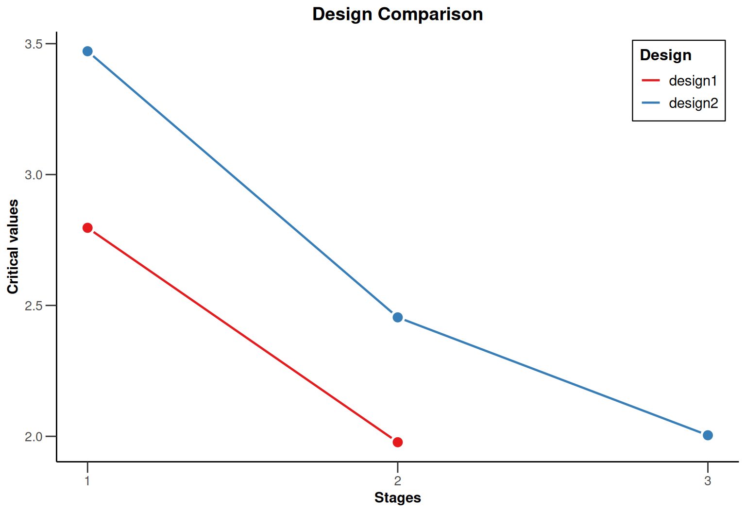
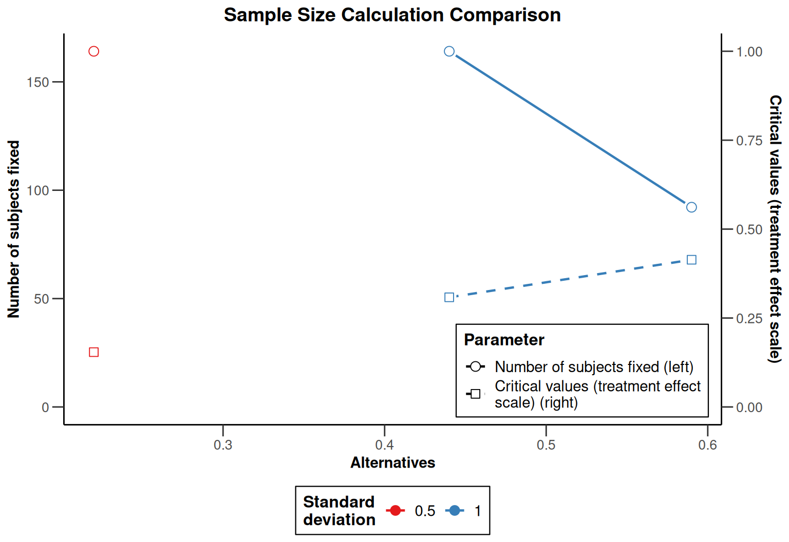
xAxis selects the column for the horizontal axis; yAxis selects one or more numeric columns for the vertical axis. Use category to distinguish scenarios and group for an additional grouping. For example:
getSampleSizeMeans(alternative = 0.22, stDev = 0.5) |>
    compare(getSampleSizeMeans(alternative = 0.44, stDev = 1)) |>
    compare(getSampleSizeMeans(alternative = 0.59, stDev = 1)) |>
    plot(
        xAxis = "alternative",
        yAxis = c("nFixed", "criticalValuesEffectScale"),
        category = "stDev",
        plotLineEnabled = TRUE
    )
The selector can be inspected without drawing a plot or raising a plot-selection error:
selection <- comp |> getComparisonPlotParameters()
selection[c("xAxis", "yAxis", "message", "candidates")]
$xAxis
NULL
$yAxis
NULL
$message
[1] "Cannot select plot axes unambiguously.\nPlease specify xAxis and yAxis explicitly.\n\nAvailable for xAxis:\n - stages: Stages\n - kMax: Maximum number of stages\n - informationRates: Information rates\n\nAvailable for yAxis:\n - alphaSpent: Cumulative alpha spending\n - criticalValues: Critical values\n - stageLevels: Stage levels (one-sided)\n - information: Informations\n - power: Power\n ... and 1 more.\n\nExample:\n plot(x,\n xAxis = \"stages\",\n yAxis = \"alphaSpent\")"
$candidates
$candidates$xAxis
[1] "stages" "kMax" "informationRates"
$candidates$yAxis
[1] "alphaSpent" "criticalValues" "stageLevels"
[4] "information" "power" "rejectionProbabilities"
$candidates$category
[1] "objectName" "objectNumber"
$candidates$group
[1] "objectNumber" "objectName" "stages"
[4] "situation" "objectType" "endpoint"
[7] "calculationTarget" "kMax" "informationRates"
[10] "typeOfDesign" "alpha" "beta"
[13] "futilityBounds" "bindingFutility" "sided"
[16] "tolerance" "alphaSpent" "criticalValues"
[19] "stageLevels" "inflationFactor" "information"
[22] "power" "rejectionProbabilities" "futilityProbabilities"
[25] "averageSampleNumber1" "averageSampleNumber01" "averageSampleNumber0" comp |> names()[1] "design1" "design2"message is NULL when the selection is resolved. The names shown here are the identifiers supplied with add().
Consider a randomized superiority trial comparing an antihypertensive treatment with control. The endpoint is the reduction in systolic blood pressure from baseline to the assessment visit, in mmHg. We define reduction as baseline minus follow-up, so that a larger positive reduction is better. Thus alternative = 5 means a mean reduction that is 5 mmHg greater with treatment than with control. Group 1 is treatment and group 2 is control.
We initially assume:
normalApproximation = FALSE).The target effect is 5 mmHg. Effects of 4, 6, and 7 mmHg are included to assess sensitivity. We also consider a standard deviation of 15 mmHg and a 2:1 allocation, which might be attractive if more treatment exposure is desired.
fixedDesign <- getDesignFixed(alpha = 0.025, beta = 0.10, sided = 1)
planningEffects <- c(4, 5, 6, 7)

fixedPlans <- getComparison()
fixedPlans |> add(
    sd12_equal = getSampleSizeMeans(
        fixedDesign, alternative = planningEffects, stDev = 12,
        allocationRatioPlanned = 1
    )
)
Sample size calculation comparison
1 objects; 4 comparison rows; 25 columns.
Object types
Observed metrics (across objects, stages and situations)
Available operations
fixedPlans |> add(
    sd15_equal = getSampleSizeMeans(
        fixedDesign, alternative = planningEffects, stDev = 15,
        allocationRatioPlanned = 1
    )
)
Sample size calculation comparison
2 objects; 8 comparison rows; 25 columns.
Object types
Observed metrics (across objects, stages and situations)
Available operations
fixedPlans |> add(
    sd12_2to1 = getSampleSizeMeans(
        fixedDesign, alternative = planningEffects, stDev = 12,
        allocationRatioPlanned = 2
    )
)
Sample size calculation comparison
3 objects; 12 comparison rows; 25 columns.
Object types
Observed metrics (across objects, stages and situations)
Available operations
print(fixedPlans)Sample size calculation comparison
3 objects; 12 comparison rows; 25 columns.
Object types
Observed metrics (across objects, stages and situations)
Available operations
summary(fixedPlans, digits = 3, maxParameters = 20, maxProfiles = 4)Sample size calculation comparison summary
Comparison of 3 sample size means calculations. The comparison identifies 6 differing parameters and 15 shared parameters or profiles. Shared (examples): Object type, Endpoint, Calculation target, Alternatives, Type II error rate, Normal approximation, … (all shared captions: showAll = TRUE)
Inputs and design settings
Standard deviation - integer, factor [2 profiles]
| Parameter | Value |
|---|---|
| sd12_equal, sd12_2to1 | 12 |
| sd15_equal | 15 |
Planned allocation ratio - integer, factor [2 profiles]
| Parameter | Value |
|---|---|
| sd12_equal, sd15_equal | 1 |
| sd12_2to1 | 2 |
Results and derived parameters
Critical values (treatment effect scale) - numeric, continuous [3 profiles]
| Parameter | Situation 1 | Situation 2 | Situation 3 | Situation 4 |
|---|---|---|---|---|
| sd12_equal | 2.42 | 3.026 | 3.633 | 4.241 |
| sd15_equal | 2.42 | 3.025 | 3.631 | 4.238 |
| sd12_2to1 | 2.42 | 3.026 | 3.633 | 4.24 |
Number of subjects fixed - numeric, continuous [3 profiles]
| Parameter | Situation 1 | Situation 2 | Situation 3 | Situation 4 |
|---|---|---|---|---|
| sd12_equal | 380.198 | 244.028 | 170.063 | 125.468 |
| sd15_equal | 592.97 | 380.198 | 264.621 | 194.934 |
| sd12_2to1 | 427.481 | 274.287 | 191.075 | 140.904 |
Number of subjects fixed (1) - numeric, continuous [3 profiles]
| Parameter | Situation 1 | Situation 2 | Situation 3 | Situation 4 |
|---|---|---|---|---|
| sd12_equal | 190.099 | 122.014 | 85.031 | 62.734 |
| sd15_equal | 296.485 | 190.099 | 132.311 | 97.467 |
| sd12_2to1 | 284.987 | 182.858 | 127.383 | 93.936 |
Number of subjects fixed (2) - numeric, continuous [3 profiles]
| Parameter | Situation 1 | Situation 2 | Situation 3 | Situation 4 |
|---|---|---|---|---|
| sd12_equal | 190.099 | 122.014 | 85.031 | 62.734 |
| sd15_equal | 296.485 | 190.099 | 132.311 | 97.467 |
| sd12_2to1 | 142.494 | 91.429 | 63.692 | 46.968 |
Legend
Complete display: summary(x, showAll = TRUE). Full data: as.data.frame(x). Exact profiles: summary(x)$parameterInfo.
Each object contains several situations, one per effect assumption. The comparison retains both the object identity and the situations within it. The summary helps check that the intended assumptions differ while the significance level and target power are shared. Display limits can be increased for a fuller overview; they do not truncate the data frame.
fixedData <- as.data.frame(fixedPlans)
fixedTable <- fixedData[, c(
    "objectName", "alternative", "stDev", "allocationRatioPlanned",
    "nFixed", "nFixed1", "nFixed2"
)]
knitr::kable(fixedTable, digits = 1, row.names = FALSE)| objectName | alternative | stDev | allocationRatioPlanned | nFixed | nFixed1 | nFixed2 |
|---|---|---|---|---|---|---|
| sd12_equal | 4 | 12 | 1 | 380.2 | 190.1 | 190.1 |
| sd12_equal | 5 | 12 | 1 | 244.0 | 122.0 | 122.0 |
| sd12_equal | 6 | 12 | 1 | 170.1 | 85.0 | 85.0 |
| sd12_equal | 7 | 12 | 1 | 125.5 | 62.7 | 62.7 |
| sd15_equal | 4 | 15 | 1 | 593.0 | 296.5 | 296.5 |
| sd15_equal | 5 | 15 | 1 | 380.2 | 190.1 | 190.1 |
| sd15_equal | 6 | 15 | 1 | 264.6 | 132.3 | 132.3 |
| sd15_equal | 7 | 15 | 1 | 194.9 | 97.5 | 97.5 |
| sd12_2to1 | 4 | 12 | 2 | 427.5 | 285.0 | 142.5 |
| sd12_2to1 | 5 | 12 | 2 | 274.3 | 182.9 | 91.4 |
| sd12_2to1 | 6 | 12 | 2 | 191.1 | 127.4 | 63.7 |
| sd12_2to1 | 7 | 12 | 2 | 140.9 | 93.9 | 47.0 |
nFixed is the total sample size, and nFixed1 and nFixed2 are the group-specific sizes. The calculations return fractional requirements; an operational plan needs integer group sizes. For a quick comparison of how sample size changes with the assumed effect:
plot(fixedPlans, xAxis = "alternative", yAxis = "nFixed")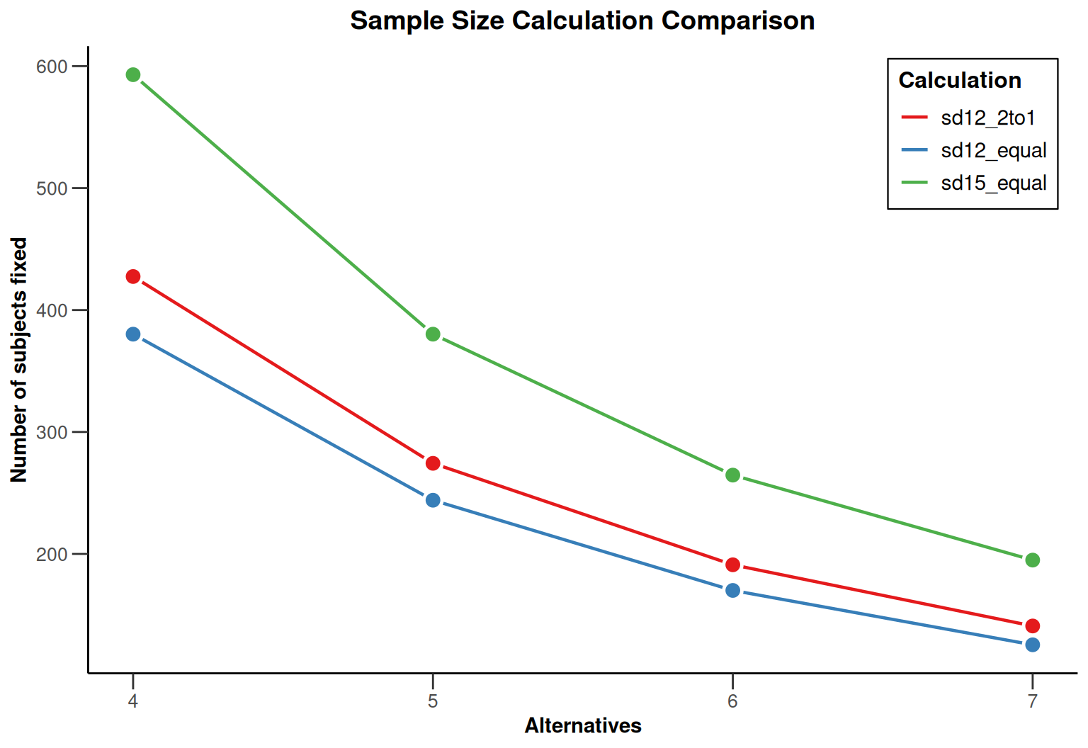
The smaller effect requires substantially more patients. Higher variability also increases the requirement. With equal variances and otherwise identical assumptions, 2:1 allocation is less efficient in terms of total sample size than 1:1 allocation. The curves make this cost visible before deciding whether the additional treatment exposure justifies it.
Suppose the team selects the 5 mmHg effect, standard deviation 12 mmHg, and equal allocation. We retrieve the corresponding object and round the group size upward:
referencePlan <- fixedPlans |> fetch("sd12_equal")
referenceSituation <- match(5, referencePlan$alternative)
subjectsPerGroup <- ceiling(referencePlan$nFixed1[referenceSituation])
fixedTotal <- 2 * subjectsPerGroup

data.frame(subjectsPerGroup, fixedTotal)
subjectsPerGroup fixedTotal
1 123 246The resulting plan has 123 evaluable patients per group, or 246 in total. If 10% of randomized patients are expected to have no usable endpoint, a simple recruitment allowance would be 274 patients, rounding within each group. The power calculations below use the evaluable sample size, not the larger recruitment target. This allowance is a planning simplification and does not specify the analysis of missing outcomes.
Now hold the selected total sample size fixed and calculate power under several possible true effects. Recalculating the sample size for each effect would answer a different question.
powerEffects <- seq(3, 7, by = 0.5)
fixedPower <- getComparison()
fixedPower |> add(
    sd12_equal = getPowerMeans(
        fixedDesign, alternative = powerEffects, stDev = 12,
        allocationRatioPlanned = 1, maxNumberOfSubjects = fixedTotal
    )
)
Power calculation comparison
1 objects; 9 comparison rows; 28 columns.
Object types
Observed metrics (across objects, stages and situations)
Available operations
fixedPower |> add(
    sd15_equal = getPowerMeans(
        fixedDesign, alternative = powerEffects, stDev = 15,
        allocationRatioPlanned = 1, maxNumberOfSubjects = fixedTotal
    )
)
Power calculation comparison
2 objects; 18 comparison rows; 28 columns.
Object types
Observed metrics (across objects, stages and situations)
Available operations
fixedPower |> add(
    sd12_2to1 = getPowerMeans(
        fixedDesign, alternative = powerEffects, stDev = 12,
        allocationRatioPlanned = 2, maxNumberOfSubjects = fixedTotal
    )
)
Power calculation comparison
3 objects; 27 comparison rows; 28 columns.
Object types
Observed metrics (across objects, stages and situations)
Available operations
print(fixedPower)Power calculation comparison
3 objects; 27 comparison rows; 28 columns.
Object types
Observed metrics (across objects, stages and situations)
Available operations
summary(fixedPower, digits = 3, maxParameters = 20)Power calculation comparison summary
Comparison of 3 power means calculations. The comparison identifies 6 differing parameters and 18 shared parameters or profiles. Shared (examples): Object type, Endpoint, Calculation target, Alternatives, Maximum number of subjects, Type II error rate, … (all shared captions: showAll = TRUE)
Inputs and design settings
Standard deviation - integer, factor [2 profiles]
| Parameter | Value |
|---|---|
| sd12_equal, sd12_2to1 | 12 |
| sd15_equal | 15 |
Planned allocation ratio - integer, factor [2 profiles]
| Parameter | Value |
|---|---|
| sd12_equal, sd15_equal | 1 |
| sd12_2to1 | 2 |
Results and derived parameters
Overall reject - numeric, continuous [3 profiles]
| Parameter | Situation 1 | Situation 2 | Situation 3 | Situation 4 | … |
|---|---|---|---|---|---|
| sd12_equal | 0.497 | 0.625 | 0.74 | 0.834 | … (+5 values; increase maxValues) |
| sd15_equal | 0.345 | 0.445 | 0.549 | 0.649 | … (+5 values; increase maxValues) |
| sd12_2to1 | 0.453 | 0.575 | 0.69 | 0.789 | … (+5 values; increase maxValues) |
Critical values (treatment effect scale) - numeric, continuous [3 profiles]
| Parameter | Value |
|---|---|
| sd12_equal | 3.014 |
| sd15_equal | 3.768 |
| sd12_2to1 | 3.197 |
Number of subjects fixed (1) - integer, factor [2 profiles]
| Parameter | Value |
|---|---|
| sd12_equal, sd15_equal | 123 |
| sd12_2to1 | 164 |
Number of subjects fixed (2) - integer, factor [2 profiles]
| Parameter | Value |
|---|---|
| sd12_equal, sd15_equal | 123 |
| sd12_2to1 | 82 |
Legend
Complete display: summary(x, showAll = TRUE). Full data: as.data.frame(x). Exact profiles: summary(x)$parameterInfo.
For a concise decision table, retain the target and a smaller effect:
fixedPowerData <- as.data.frame(fixedPower)
knitr::kable(
    subset(fixedPowerData, alternative %in% c(4, 5), select = c(
        objectName, alternative, stDev, allocationRatioPlanned,
        maxNumberOfSubjects, overallReject
    )),
    digits = 3, row.names = FALSE
)| objectName | alternative | stDev | allocationRatioPlanned | maxNumberOfSubjects | overallReject |
|---|---|---|---|---|---|
| sd12_equal | 4 | 12 | 1 | 246 | 0.740 |
| sd12_equal | 5 | 12 | 1 | 246 | 0.902 |
| sd15_equal | 4 | 15 | 1 | 246 | 0.549 |
| sd15_equal | 5 | 15 | 1 | 246 | 0.740 |
| sd12_2to1 | 4 | 12 | 2 | 246 | 0.690 |
| sd12_2to1 | 5 | 12 | 2 | 246 | 0.866 |
plot(fixedPower, xAxis = "alternative", yAxis = "overallReject") +
    geom_hline(yintercept = 0.90, linetype = "dashed", colour = "grey40")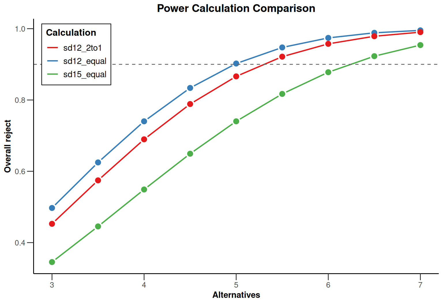
overallReject is the probability of rejecting the null hypothesis. At 5 mmHg, the reference scenario reaches at least 90% power after rounding. A smaller effect, higher standard deviation, or unequal allocation at this same total can reduce power. This calculation checks consistency with the planning assumptions; it is not independent validation of the statistical model or software.
We now consider an interim analysis at 50% information, followed by the final analysis. All sequential designs use the same one-sided alpha-spending O’Brien-Fleming efficacy rule (typeOfDesign = "asOF"), significance level, and target power. Only the interim futility rule changes:
| Scenario | Interim futility rule | Planning interpretation |
|---|---|---|
no_futility |
No futility stopping | Continue unless efficacy is established. |
z0 |
Stop if the interim Z statistic is below 0 | Stop for an effect in the unfavorable direction. |
z0_5 |
Stop if Z is below 0.5 | Require at least a modest favorable signal to continue. |
z1 |
Stop if Z is below 1 | A more demanding continuation rule, with greater risk of discarding an effective treatment. |
These are candidate rules for discussion with the study team. Their one-sided p-value thresholds are 0.50, approximately 0.31, and approximately 0.16, respectively; they are not conditional-power thresholds. The corresponding thresholds in mmHg depend on information, sample size, and variability and can be inspected in the sample size plans.
We specify non-binding futility. The efficacy boundaries control the Type I error even if a futility recommendation is not followed. However, the power and expected sample size calculations below assume that the stated futility stopping rule is followed. Ignoring it changes those operating characteristics.
futilityRules <- c(no_futility = -Inf, z0 = 0, z0_5 = 0.5, z1 = 1)
sequentialDesigns <- lapply(futilityRules, function(bound) {
    binding <- if (is.finite(bound)) {
        FALSE
    } else {
        NA
    }
    return(getDesignGroupSequential(
        kMax = 2, informationRates = c(0.5, 1),
        alpha = 0.025, beta = 0.10, sided = 1,
        typeOfDesign = "asOF", futilityBounds = bound,
        bindingFutility = binding
    ))
})

designComparison <- getComparison()
designComparison |> add(objects = sequentialDesigns)
Design comparison
4 objects; 8 comparison rows; 20 columns.
Object types
Observed metrics (across objects, stages and situations)
Available operations
summary(designComparison, digits = 3, maxParameters = 20, maxProfiles = 4)Design comparison summary
Comparison of 4 trial planning results: group sequential design. The comparison identifies 1 differing parameter and 15 shared parameters or profiles. Shared (examples): Object type, Endpoint, Calculation target, Type of design, Type II error rate, Information rates, … (all shared captions: showAll = TRUE)
Inputs and design settings
Futility bounds (non-binding) - numeric, continuous [4 profiles]
| Parameter | Value |
|---|---|
| no_futility | -Inf |
| z0 | 0 |
| z0_5 | 0.5 |
| z1 | 1 |
Legend
Complete display: summary(x, showAll = TRUE). Full data: as.data.frame(x). Exact profiles: summary(x)$parameterInfo.
Since the designs are already available as a named list, pass the entire list to add() in one call. Its entries are added in list order and retain their names; there is no need for another loop. You can also pass the list directly to the constructor with getComparison(objects = sequentialDesigns).
The design summary checks that the efficacy settings agree and that the futility bounds differ as intended. -Inf disables futility stopping at the interim analysis.
For each design, calculate the sample size needed for 90% power at effects of 4, 5, and 6 mmHg, using standard deviation 12 mmHg and equal allocation:
sequentialPlans <- getComparison()
for (scenarioName in names(designComparison)) {
    design <- designComparison |> fetch(scenarioName)
    plan <- getSampleSizeMeans(
        design, alternative = c(4, 5, 6), stDev = 12,
        allocationRatioPlanned = 1
    )
    sequentialPlans |> add(objects = setNames(list(plan), scenarioName))
}

print(sequentialPlans)
Sample size calculation comparison
4 objects; 24 comparison rows; 42 columns.
Object types
Observed metrics (across objects, stages and situations)
Available operations
summary(sequentialPlans, digits = 3, maxParameters = 25, maxProfiles = 4)Sample size calculation comparison summary
Comparison of 4 sample size means calculations. The comparison identifies 15 differing parameters and 23 shared parameters or profiles. Shared (examples): Object type, Endpoint, Calculation target, Alternatives, Standard deviation, Type of design, … (all shared captions: showAll = TRUE)
Inputs and design settings
Futility bounds (non-binding) - numeric, continuous [4 profiles]
| Parameter | Value |
|---|---|
| no_futility | -Inf |
| z0 | 0 |
| z0_5 | 0.5 |
| z1 | 1 |
Results and derived parameters
Maximum number of subjects - numeric, continuous [4 profiles]
| Parameter | Situation 1 | Situation 2 | Situation 3 |
|---|---|---|---|
| no_futility | 381.498 | 244.862 | 170.644 |
| z0 | 384.609 | 246.859 | 172.036 |
| z0_5 | 399.003 | 256.097 | 178.474 |
| z1 | 450.183 | 288.947 | 201.367 |
Maximum number of subjects (1) - numeric, continuous [4 profiles]
| Parameter | Situation 1 | Situation 2 | Situation 3 |
|---|---|---|---|
| no_futility | 190.749 | 122.431 | 85.322 |
| z0 | 192.305 | 123.429 | 86.018 |
| z0_5 | 199.501 | 128.049 | 89.237 |
| z1 | 225.091 | 144.474 | 100.683 |
Maximum number of subjects (2) - numeric, continuous [4 profiles]
| Parameter | Situation 1 | Situation 2 | Situation 3 |
|---|---|---|---|
| no_futility | 190.749 | 122.431 | 85.322 |
| z0 | 192.305 | 123.429 | 86.018 |
| z0_5 | 199.501 | 128.049 | 89.237 |
| z1 | 225.091 | 144.474 | 100.683 |
Number of subjects - numeric, continuous [4 profiles]
| Parameter | Stage 1 Situation 1 | Stage 1 Situation 2 | Stage 1 Situation 3 | Stage 2 Situation 1 | … |
|---|---|---|---|---|---|
| no_futility | 190.749 | 122.431 | 85.322 | 381.498 | … (+2 values; increase maxValues) |
| z0 | 192.305 | 123.429 | 86.018 | 384.609 | … (+2 values; increase maxValues) |
| z0_5 | 199.501 | 128.049 | 89.237 | 399.003 | … (+2 values; increase maxValues) |
| z1 | 225.091 | 144.474 | 100.683 | 450.183 | … (+2 values; increase maxValues) |
Expected number of subjects under H0 - numeric, continuous [4 profiles]
| Parameter | Situation 1 | Situation 2 | Situation 3 |
|---|---|---|---|
| no_futility | 381.207 | 244.675 | 170.514 |
| z0 | 288.164 | 184.956 | 128.896 |
| z0_5 | 260.751 | 167.361 | 116.634 |
| z1 | 260.46 | 167.175 | 116.504 |
Expected number of subjects under H0/H1 - numeric, continuous [4 profiles]
| Parameter | Situation 1 | Situation 2 | Situation 3 |
|---|---|---|---|
| no_futility | 374.861 | 240.602 | 167.675 |
| z0 | 353.903 | 227.15 | 158.301 |
| z0_5 | 341.749 | 219.349 | 152.864 |
| z1 | 349.893 | 224.577 | 156.507 |
Reject per stage - numeric, continuous [4 profiles]
| Parameter | Stage 1 | Stage 2 |
|---|---|---|
| no_futility | 0.253 | 0.647 |
| z0 | 0.256 | 0.644 |
| z0_5 | 0.269 | 0.631 |
| z1 | 0.32 | 0.58 |
Futility stop - numeric, continuous [4 profiles]
| Parameter | Value | Stage 1 | Stage 2 |
|---|---|---|---|
| no_futility | NA | ||
| z0 | 0.011 | NA | |
| z0_5 | 0.032 | NA | |
| z1 | 0.068 | NA |
Overall futility stop - numeric, continuous [4 profiles]
| Parameter | Value |
|---|---|
| no_futility | NA |
| z0 | 0.011 |
| z0_5 | 0.032 |
| z1 | 0.068 |
Early stop - numeric, continuous [4 profiles]
| Parameter | Value |
|---|---|
| no_futility | 0.253 |
| z0 | 0.266 |
| z0_5 | 0.302 |
| z1 | 0.387 |
Critical values (treatment effect scale) - numeric, continuous [4 profiles]
| Parameter | Stage 1 Situation 1 | Stage 1 Situation 2 | Stage 1 Situation 3 | Stage 2 Situation 1 | … |
|---|---|---|---|---|---|
| no_futility | 5.216 | 6.559 | 7.93 | 2.427 | … (+2 values; increase maxValues) |
| z0 | 5.194 | 6.531 | 7.895 | 2.417 | … (+2 values; increase maxValues) |
| z0_5 | 5.097 | 6.407 | 7.743 | 2.373 | … (+2 values; increase maxValues) |
| z1 | 4.792 | 6.019 | 7.266 | 2.233 | … (+2 values; increase maxValues) |
Futility bounds (treatment effect scale) - numeric, continuous [4 profiles]
| Parameter | Value | Stage 1 | Stage 2 | Stage 1 Situation 1 | Stage 1 Situation 2 | Stage 1 Situation 3 | Stage 2 Situation 1 | … |
|---|---|---|---|---|---|---|---|---|
| no_futility | NA | |||||||
| z0 | 0 | NA | ||||||
| z0_5 | 0.851 | 1.063 | 1.275 | NA | … (+2 values; increase maxValues) | |||
| z1 | 1.603 | 2.004 | 2.404 | NA | … (+2 values; increase maxValues) |
Futility bounds (one-sided p-value scale) - numeric, continuous [4 profiles]
| Parameter | Value | Stage 1 | Stage 2 |
|---|---|---|---|
| no_futility | NA | ||
| z0 | 0.5 | NA | |
| z0_5 | 0.309 | NA | |
| z1 | 0.159 | NA |
Expected number of subjects - numeric, continuous [4 profiles]
| Parameter | Situation 1 | Situation 2 | Situation 3 |
|---|---|---|---|
| no_futility | 333.33 | 213.946 | 149.098 |
| z0 | 333.439 | 214.016 | 149.147 |
| z0_5 | 338.805 | 217.46 | 151.548 |
| z1 | 363.004 | 232.992 | 162.372 |
Legend
Complete display: summary(x, showAll = TRUE). Full data: as.data.frame(x). Exact profiles: summary(x)$parameterInfo.
Here the loop calculates a new plan and adds it immediately. In this case, setNames(list(plan), scenarioName) supplies the scenario name programmatically. add(objects = ...) retains the list entry’s name; add(scenarioName = plan) would instead use the literal name "scenarioName".
For a sequential trial, distinguish the maximum sample size, which determines the recruitment commitment if the study continues, from the expected sample size, which averages over early stopping. A stronger futility rule can require a larger maximum sample size to preserve the target power, even while reducing expected recruitment under an ineffective treatment.
The comparison data have one row per stage and situation. Overall results are repeated across stages, while quantities such as numberOfSubjects and rejectPerStage are stage-specific. For a table of overall sample size requirements, select the final-stage rows rather than adding the repeated totals:
sequentialData <- as.data.frame(sequentialPlans)
sequentialTotals <- subset(sequentialData, stages == kMax)
knitr::kable(
    subset(sequentialTotals, alternative == 5, select = c(
        objectName,
        alternative,
        maxNumberOfSubjects,
        expectedNumberOfSubjects
    )),
    digits = 1, row.names = FALSE
)| objectName | alternative | maxNumberOfSubjects | expectedNumberOfSubjects |
|---|---|---|---|
| no_futility | 5 | 244.9 | 213.9 |
| z0 | 5 | 246.9 | 214.0 |
| z0_5 | 5 | 256.1 | 217.5 |
| z1 | 5 | 288.9 | 233.0 |
For reference, the fixed design at 5 mmHg required 244 patients before rounding and has no early stopping benefit.
plot(
    sequentialPlans,
    xAxis = "alternative",
    yAxis = c("maxNumberOfSubjects", "expectedNumberOfSubjects"),
    yAxisSide = "left",
    main = "Maximum and expected sample size"
) +
    labs(y = "Total sample size (patients)")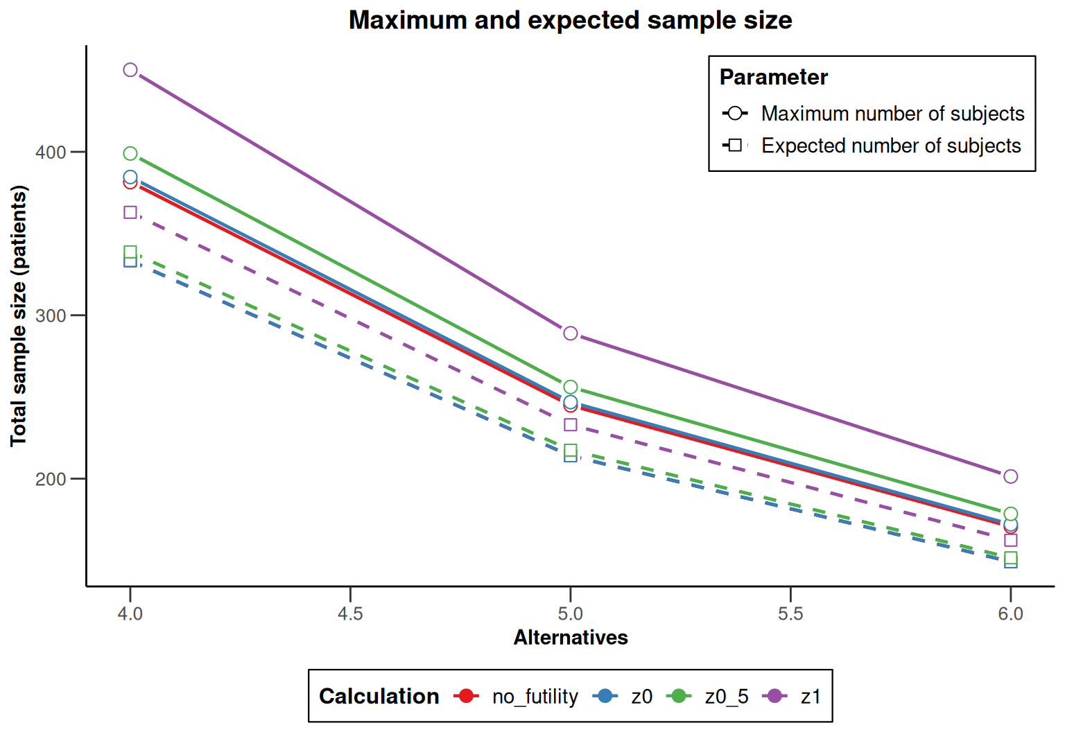
Both plotted quantities use the same unit, patients, and the same axis. The line types distinguish the maximum from the expected size. A design decision should consider both, together with the expected size under the null shown in the table.
First validate each strategy at its own rounded maximum sample size, keeping the 50% information analysis and equal allocation. This checks that re-planning has compensated for the power cost of futility.
roundedMaxima <- vapply(getObjects(sequentialPlans), function(plan) {
    situation <- match(5, plan$alternative)
    return(2 * ceiling(plan$maxNumberOfSubjects[situation] / 2))
}, numeric(1))

sequentialValidation <- getComparison()
for (scenarioName in names(designComparison)) {
    validation <- getPowerMeans(
        designComparison |> fetch(scenarioName), alternative = 5, stDev = 12,
        allocationRatioPlanned = 1,
        maxNumberOfSubjects = roundedMaxima[[scenarioName]]
    )
    sequentialValidation |> add(objects = setNames(list(validation), scenarioName))
}
validationData <- as.data.frame(sequentialValidation)

knitr::kable(
    subset(validationData, stages == kMax, select = c(
        objectName, maxNumberOfSubjects, overallReject,
        expectedNumberOfSubjects, futilityStop
    )),
    digits = 3, row.names = FALSE
)| objectName | maxNumberOfSubjects | overallReject | expectedNumberOfSubjects | futilityStop |
|---|---|---|---|---|
| no_futility | 246 | 0.901 | 214.727 | NA |
| z0 | 248 | 0.901 | 214.805 | 0.010 |
| z0_5 | 258 | 0.902 | 218.767 | 0.032 |
| z1 | 290 | 0.901 | 233.638 | 0.067 |
At the target effect, all strategies should reach at least 90% power, subject to numerical precision. The calculation retains the specified information fractions. In an operational plan, round the interim group sizes as well and check the resulting information fractions if they change materially. For the short assessment window assumed here, recruitment can be paused for the interim decision; patients already recruited but awaiting outcomes would need additional planning if that assumption is unrealistic.
The previous comparison allowed the maximum sample size to differ. A complementary question is: What would each stopping rule achieve with the same recruitment budget? Suppose the team can support the rounded maximum required by the z0_5 design at 5 mmHg. Hold that maximum fixed for every rule and vary the true effect, including zero.
commonMaximum <- roundedMaxima[["z0_5"]]
sequentialPower <- getComparison()
for (scenarioName in names(designComparison)) {
    power <- getPowerMeans(
        designComparison |> fetch(scenarioName),
        alternative = seq(0, 7, by = 0.5), stDev = 12,
        allocationRatioPlanned = 1, maxNumberOfSubjects = commonMaximum
    )
    sequentialPower |> add(objects = setNames(list(power), scenarioName))
}

print(sequentialPower)
Power calculation comparison
4 objects; 120 comparison rows; 40 columns.
Object types
Observed metrics (across objects, stages and situations)
Available operations
summary(sequentialPower, digits = 3, maxParameters = 25, maxProfiles = 4)Power calculation comparison summary
Comparison of 4 power means calculations. The comparison identifies 9 differing parameters and 27 shared parameters or profiles. Shared (examples): Object type, Endpoint, Calculation target, Alternatives, Standard deviation, Maximum number of subjects, … (all shared captions: showAll = TRUE)
Inputs and design settings
Futility bounds (non-binding) - numeric, continuous [4 profiles]
| Parameter | Value |
|---|---|
| no_futility | -Inf |
| z0 | 0 |
| z0_5 | 0.5 |
| z1 | 1 |
Results and derived parameters
Expected number of subjects - numeric, continuous [4 profiles]
| Parameter | Situation 1 | Situation 2 | Situation 3 | Situation 4 | … |
|---|---|---|---|---|---|
| no_futility | 257.803 | 257.588 | 257.179 | 256.445 | … (+11 values; increase maxValues) |
| z0 | 193.303 | 205.108 | 216.072 | 225.521 | … (+11 values; increase maxValues) |
| z0_5 | 168.605 | 179.644 | 191.211 | 202.533 | … (+11 values; increase maxValues) |
| z1 | 149.27 | 157.271 | 166.694 | 177.089 | … (+11 values; increase maxValues) |
Reject per stage - numeric, continuous [4 profiles]
| Parameter | Stage 1 Situation 1 | Stage 1 Situation 2 | Stage 1 Situation 3 | Stage 1 Situation 4 | … |
|---|---|---|---|---|---|
| no_futility | 0.002 | 0.003 | 0.006 | 0.012 | … (+26 values; increase maxValues) |
| z0 | 0.002 | 0.003 | 0.006 | 0.012 | … (+26 values; increase maxValues) |
| z0_5 | 0.002 | 0.003 | 0.006 | 0.012 | … (+26 values; increase maxValues) |
| z1 | 0.002 | 0.003 | 0.006 | 0.012 | … (+26 values; increase maxValues) |
Overall reject - numeric, continuous [4 profiles]
| Parameter | Situation 1 | Situation 2 | Situation 3 | Situation 4 | … |
|---|---|---|---|---|---|
| no_futility | 0.025 | 0.052 | 0.098 | 0.168 | … (+11 values; increase maxValues) |
| z0 | 0.025 | 0.051 | 0.097 | 0.166 | … (+11 values; increase maxValues) |
| z0_5 | 0.024 | 0.049 | 0.093 | 0.16 | … (+11 values; increase maxValues) |
| z1 | 0.02 | 0.043 | 0.081 | 0.141 | … (+11 values; increase maxValues) |
Futility stop - numeric, continuous [4 profiles]
| Parameter | Value | Stage 1 Situation 1 | Stage 1 Situation 2 | Stage 1 Situation 3 | Stage 1 Situation 4 | … |
|---|---|---|---|---|---|---|
| no_futility | NA | |||||
| z0 | 0.5 | 0.407 | 0.319 | 0.24 | … (+26 values; increase maxValues) | |
| z0_5 | 0.691 | 0.604 | 0.511 | 0.418 | … (+26 values; increase maxValues) | |
| z1 | 0.841 | 0.778 | 0.701 | 0.615 | … (+26 values; increase maxValues) |
Overall futility stop - numeric, continuous [4 profiles]
| Parameter | Value | Situation 1 | Situation 2 | Situation 3 | Situation 4 | … |
|---|---|---|---|---|---|---|
| no_futility | NA | |||||
| z0 | 0.5 | 0.407 | 0.319 | 0.24 | … (+11 values; increase maxValues) | |
| z0_5 | 0.691 | 0.604 | 0.511 | 0.418 | … (+11 values; increase maxValues) | |
| z1 | 0.841 | 0.778 | 0.701 | 0.615 | … (+11 values; increase maxValues) |
Early stop - numeric, continuous [4 profiles]
| Parameter | Situation 1 | Situation 2 | Situation 3 | Situation 4 | … |
|---|---|---|---|---|---|
| no_futility | 0.002 | 0.003 | 0.006 | 0.012 | … (+11 values; increase maxValues) |
| z0 | 0.502 | 0.41 | 0.325 | 0.252 | … (+11 values; increase maxValues) |
| z0_5 | 0.693 | 0.607 | 0.518 | 0.43 | … (+11 values; increase maxValues) |
| z1 | 0.843 | 0.781 | 0.708 | 0.627 | … (+11 values; increase maxValues) |
Futility bounds (treatment effect scale) - numeric, continuous [4 profiles]
| Parameter | Value | Stage 1 | Stage 2 |
|---|---|---|---|
| no_futility | NA | ||
| z0 | 0 | NA | |
| z0_5 | 1.059 | NA | |
| z1 | 2.121 | NA |
Futility bounds (one-sided p-value scale) - numeric, continuous [4 profiles]
| Parameter | Value | Stage 1 | Stage 2 |
|---|---|---|---|
| no_futility | NA | ||
| z0 | 0.5 | NA | |
| z0_5 | 0.309 | NA | |
| z1 | 0.159 | NA |
Legend
Complete display: summary(x, showAll = TRUE). Full data: as.data.frame(x). Exact profiles: summary(x)$parameterInfo.
plot(
    sequentialPower, xAxis = "alternative", yAxis = "overallReject"
) +
    geom_hline(yintercept = 0.90, linetype = "dashed", colour = "grey40")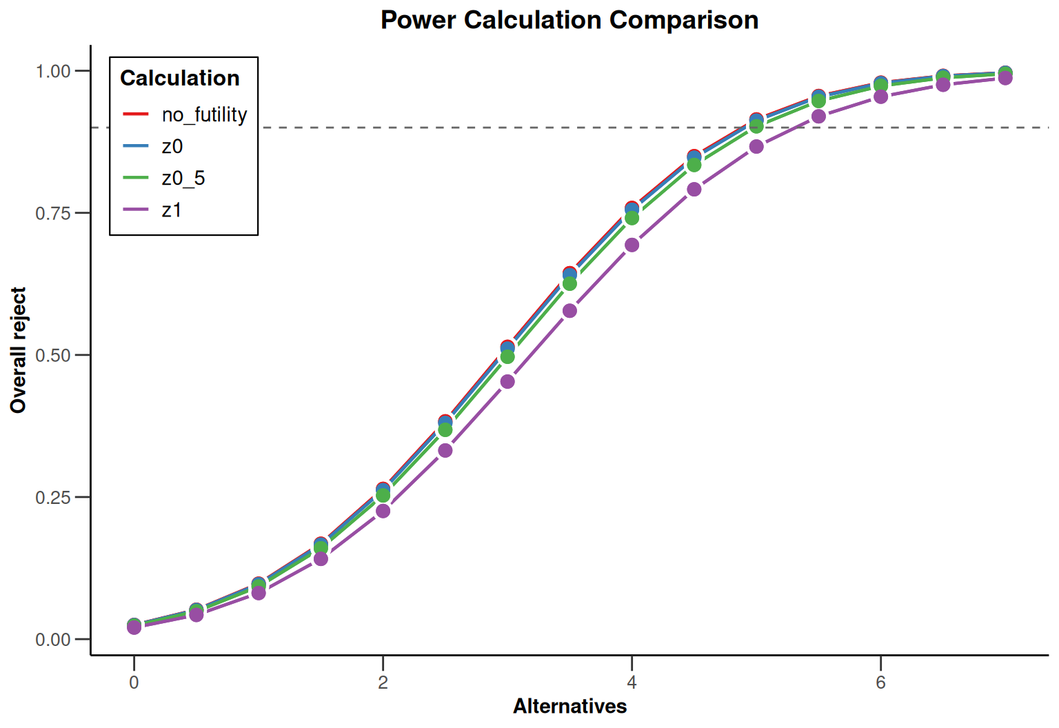
plot(
    summary(sequentialPower),
    xAxis = "alternative",
    yAxis = "expectedNumberOfSubjects"
)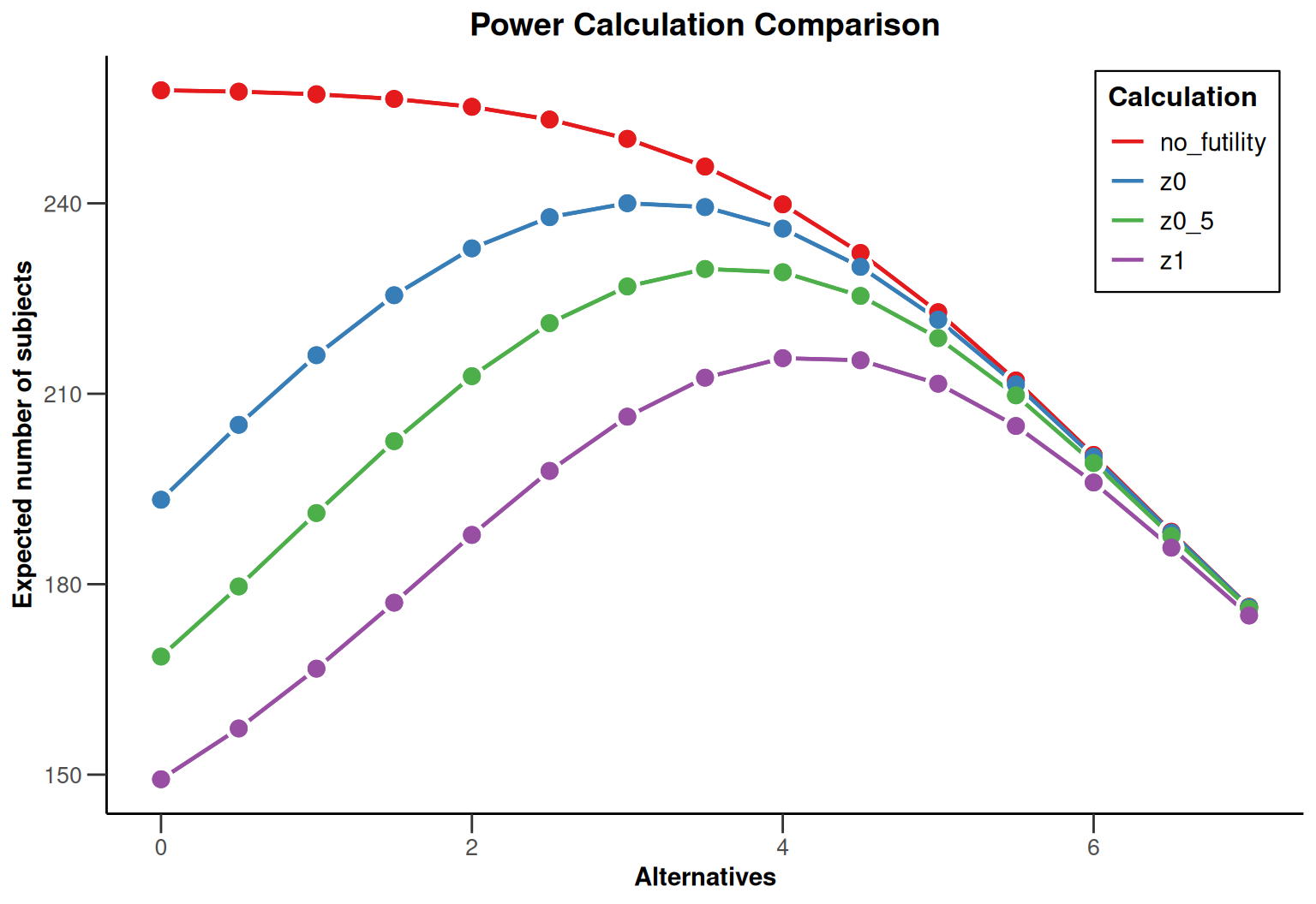
Plotting the summary uses its captured comparison data. The expected sample size can be largest at intermediate effects: a clearly ineffective treatment may stop for futility, and a large effect may stop for efficacy, while an intermediate effect often reaches the final analysis.
To support the design meeting, extract a table at the null, a smaller effect, and the target effect:
sequentialPowerData <- as.data.frame(sequentialPower)
decisionTable <- subset(
    sequentialPowerData, stages == kMax & alternative %in% c(0, 4, 5),
    select = c(
        objectName, alternative, maxNumberOfSubjects, overallReject,
        expectedNumberOfSubjects, futilityStop, earlyStop
    )
)
knitr::kable(decisionTable, digits = 3, row.names = FALSE)| objectName | alternative | maxNumberOfSubjects | overallReject | expectedNumberOfSubjects | futilityStop | earlyStop |
|---|---|---|---|---|---|---|
| no_futility | 0 | 258 | 0.025 | 257.803 | NA | 0.002 |
| no_futility | 4 | 258 | 0.759 | 239.837 | NA | 0.141 |
| no_futility | 5 | 258 | 0.914 | 222.848 | NA | 0.272 |
| z0 | 0 | 258 | 0.025 | 193.303 | 0.500 | 0.502 |
| z0 | 4 | 258 | 0.755 | 236.011 | 0.030 | 0.170 |
| z0 | 5 | 258 | 0.912 | 221.660 | 0.009 | 0.282 |
| z0_5 | 0 | 258 | 0.024 | 168.605 | 0.691 | 0.693 |
| z0_5 | 4 | 258 | 0.741 | 229.143 | 0.083 | 0.224 |
| z0_5 | 5 | 258 | 0.902 | 218.767 | 0.032 | 0.304 |
| z1 | 0 | 258 | 0.020 | 149.270 | 0.841 | 0.843 |
| z1 | 4 | 258 | 0.694 | 215.604 | 0.188 | 0.329 |
| z1 | 5 | 258 | 0.867 | 211.581 | 0.087 | 0.360 |
targetDecision <- subset(decisionTable, alternative == 5)
nullDecision <- subset(decisionTable, alternative == 0)
At zero effect, overallReject is the actual Type I error under the stated stopping policy. It can be below 0.025 when non-binding futility is followed. futilityStop is the probability of stopping early for futility; earlyStop includes both early efficacy and futility stopping. At 5 mmHg, the table shows whether the available maximum can sustain the target power for each rule. At 4 mmHg, it quantifies the consequences of an overoptimistic effect assumption.
For the design without futility, the exported futilityStop is NA because no futility rule is active. In this scenario there is no early stopping for futility; do not treat this entry as an estimated stopping probability.
With a common maximum of 258 patients, the z1 rule achieves only 86.7% power at 5 mmHg. The z0_5 rule retains 90.2% power and requires an expected 169 patients under the null, compared with 258 without futility. These figures make the recruitment benefit and the power trade-off explicit.
The z0_5 design is a candidate, not an automatically selected optimum. Compared with no futility stopping, it trades some probability of success at a common maximum for lower expected recruitment under small effects. A more demanding rule such as z1 may require a larger maximum to recover 90% power. The final choice depends on the acceptable risk of stopping an effective treatment, recruitment capacity, and the value of early termination.
The following methods complement the reporting workflow:
| Function or operator | Use in a planning workflow |
|---|---|
compare(x, y) |
Start a comparison from planning objects or append to an existing comparison in place. |
print(x) |
Inspect the collection and selected observed ranges. |
summary(x) |
Identify differing inputs, design settings, and results. |
plot(x) or plot(summary(x)) |
Plot selected results against assumptions or stages. |
as.data.frame(x) |
Export the full unrounded comparison table. |
names(x), length(x) |
Inspect scenario names and the number of contained objects. |
getObjects(x) |
Retrieve the list of contained objects. |
fetch(x, ...) |
Retrieve objects by name or position, including several selections. |
x[[i]], x[["name"]], x$name |
Access a contained object directly. |
add(x, ...), delete(x, index) |
Extend a comparison or remove one object in place. |
For example, build a shortlist without altering the collection of all fixed-design scenarios:
names(fixedPlans)[1] "sd12_equal" "sd15_equal" "sd12_2to1" length(fixedPlans)[1] 3names(getObjects(fixedPlans))[1] "sd12_equal" "sd15_equal" "sd12_2to1" identical(fixedPlans$sd12_equal, fixedPlans[["sd12_equal"]])[1] TRUEidentical(fetch(fixedPlans, 1), fixedPlans[[1]])[1] TRUEshortlist <- getComparison()
shortlist |> add(objects = fixedPlans |>
fetch(c("sd12_equal", "sd15_equal"), output = "list"))Sample size calculation comparison
2 objects; 8 comparison rows; 25 columns.
Object types
Observed metrics (across objects, stages and situations)
Available operations
shortlist |>
    add(sd12_2to1 = fixedPlans[["sd12_2to1"]]) |>
    delete("sd15_equal")
Sample size calculation comparison
2 objects; 8 comparison rows; 25 columns.
Object types
Observed metrics (across objects, stages and situations)
Available operations
names(shortlist)[1] "sd12_equal" "sd12_2to1" Comparisons retain references to their contained objects. add(), delete(), and compare() with an existing comparison modify it in place; assigning it to another variable does not create an independent collection. Construct a new comparison, as above, to make a separate shortlist. The contained plans are still shared. Existing summaries are snapshots, so call summary() again after changing a comparison. R6 member names take precedence with $; use [["name"]] if a scenario name collides with a method name.
The fixed-design comparison exposes the cost of uncertainty in effect and variability before committing to a sample size. The subsequent power comparison quantifies what happens if the selected assumptions do not hold. For the sequential trial, the equal-power sample size comparison and the common-budget power comparison answer complementary questions: the first establishes recruitment requirements, and the second shows the consequences of choosing different stopping rules within a feasible maximum.
Start directly from a planning object with |> compare(), or create a named collection with getComparison() and extend it with |> add() as scenarios become available. Use fetch() to select scenarios and delete() to refine the collection. Use print() for an initial overview, summary() to verify the intended differences, plots to examine sensitivity, and selected data-frame columns to document the decision. Record the chosen effect, standard deviation, allocation, integer sample sizes, analysis timing, and stopping policy together with the resulting power and expected recruitment.
For further background, see planning trials with a continuous endpoint and specifying futility bounds on different scales.