library(rpact)Enhanced Futility Bounds Specification with rpact
Planning
Utilities
This document describes how to specify futility bounds in adaptive and group sequential designs on different scales. Starting from a theoretical derivation, it illustrates how to use the
getFutilityBounds() function in rpact to convert futility bounds between z-value, p-value, effect size, conditional power, Bayesian predictive power, and reverse conditional power scales.
Introduction
This vignette demonstrates how to specify, transform, and work with futility bounds in rpact.
Futility stopping is an important tool in adaptive and group sequential designs, allowing early termination if accumulating data suggests that confirming the alternative hypothesis is unlikely. Traditionally, futility bounds are specified on the z-value or p-value scale, but in practice it is often desirable to express these boundaries on other scales, such as the effect size scale, conditional power, Bayesian predictive power, or the reverse conditional power.
In this vignette, you will learn:
- how futility bounds arise in classical designs,
- how
rpacthandles these boundaries across multiple scales, - how
getFutilityBounds()can translate futility bound values consistently between scales, - and how these transformations are used in real trial-planning workflows.
Current situation
See the following example of group sequential designs with futility bounds specified or calculated on the z-value scale in rpact version < 4.3.0.
getDesignGroupSequential(
    kMax = 3,
    alpha = 0.025,
    sided = 1,
    typeOfDesign = "OF",
    futilityBounds = c(0, -Inf)
) |>
    summary()
Sequential analysis with a maximum of 3 looks (group sequential design)
O’Brien & Fleming design, non-binding futility, one-sided overall significance level 2.5%, power 80%, undefined endpoint, inflation factor 1.0628, ASN H1 0.8528, ASN H01 0.8821, ASN H0 0.7059.
| Stage | 1 | 2 | 3 |
|---|---|---|---|
| Planned information rate | 33.3% | 66.7% | 100% |
| Cumulative alpha spent | 0.0003 | 0.0072 | 0.0250 |
| Stage levels (one-sided) | 0.0003 | 0.0071 | 0.0225 |
| Efficacy boundary (z-value scale) | 3.471 | 2.454 | 2.004 |
| Futility boundary (z-value scale) | 0 | -Inf | |
| Cumulative power | 0.0356 | 0.4617 | 0.8000 |
| Futility probabilities under H1 | 0.048 | 0 |
The derivation of futility bounds is possible with the use of the beta spending function approach. The following example yields similar futility bounds as in the example from above:
design <- getDesignGroupSequential(
    kMax = 3,
    alpha = 0.025,
    sided = 1,
    typeOfDesign = "asOF",
    typeBetaSpending = "bsKD",
    gammaB = 1.3,
    futilityStops = c(TRUE, FALSE)
)
design |> summary()
Sequential analysis with a maximum of 3 looks (group sequential design)
O’Brien & Fleming type alpha spending design and Kim & DeMets beta spending (gammaB = 1.3), non-binding futility, futility stops c(TRUE, FALSE), one-sided overall significance level 2.5%, power 80%, undefined endpoint, inflation factor 1.0586, ASN H1 0.8634, ASN H01 0.8829, ASN H0 0.7038.
| Stage | 1 | 2 | 3 |
|---|---|---|---|
| Planned information rate | 33.3% | 66.7% | 100% |
| Cumulative alpha spent | 0.0001 | 0.0060 | 0.0250 |
| Cumulative beta spent | 0.0479 | 0.0479 | 0.2000 |
| Stage levels (one-sided) | 0.0001 | 0.0060 | 0.0231 |
| Efficacy boundary (z-value scale) | 3.710 | 2.511 | 1.993 |
| Futility boundary (z-value scale) | -0.001 | -Inf | |
| Cumulative power | 0.0204 | 0.4370 | 0.8000 |
| Futility probabilities under H1 | 0.048 | 0 |
design |> plot()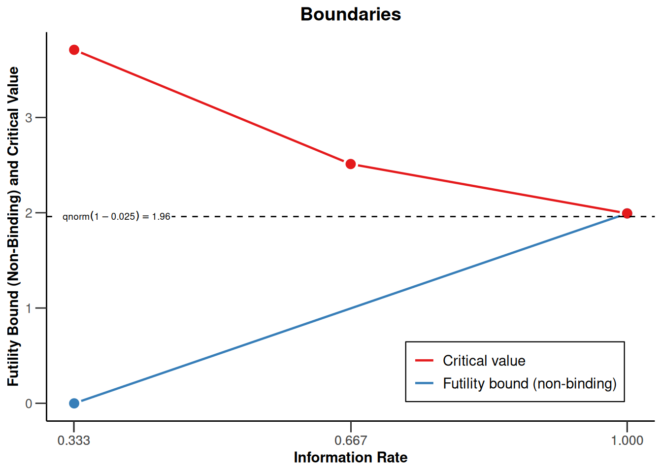
In comparison, recall how a Fisher’s combination test design is specified in rpact and how the futility boundaries look like:
getDesignFisher(
    kMax = 3,
    alpha = 0.025,
    sided = 1,
    method = "fullAlpha",
    alpha0Vec = c(0.5, 1)
) |>
    summary()
Sequential analysis with a maximum of 3 looks (Fisher’s combination test design)
Full last stage level design, binding futility, one-sided overall significance level 2.5%, undefined endpoint.
| Stage | 1 | 2 | 3 |
|---|---|---|---|
| Fixed weight | 1 | 1 | 1 |
| Cumulative alpha spent | 0.0084 | 0.0128 | 0.0250 |
| Stage levels (one-sided) | 0.0084 | 0.0084 | 0.0250 |
| Efficacy boundary (p product scale) | 0.0084123 | 0.0010734 | 0.0007284 |
| Futility boundary (separate p-value scale) | 0.5000 | 1.0000 |
The key points are:
- For group sequential designs, futility bounds have to be specified on the \(z\)-value scale. For Fisher’s combination test, they are instead specified on the separate \(p\)-value scale.
- It is desired, however, to also define futility bounds on other scales, e.g., the conditional power scale.
On the effect size scale, futility bounds are already shown in the output of the getSampleSize...() and getPower...() functions. The following example illustrates this when calculating sample sizes:
getDesignGroupSequential(
    kMax = 3,
    alpha = 0.025,
    sided = 1,
    typeOfDesign = "OF",
    futilityBounds = c(0, 0.5)
) |>
    getSampleSizeMeans(
        alternative = c(0.3, 0.5),
        normalApproximation = TRUE
    ) |>
    summary()
Sample size calculation for a continuous endpoint
Sequential analysis with a maximum of 3 looks (group sequential design), one-sided overall significance level 2.5%, power 80%. The results were calculated for a two-sample t-test (normal approximation), H0: mu(1) - mu(2) = 0, H1: effect as specified, standard deviation = 1.
| Stage | 1 | 2 | 3 |
|---|---|---|---|
| Planned information rate | 33.3% | 66.7% | 100% |
| Cumulative alpha spent | 0.0003 | 0.0072 | 0.0250 |
| Stage levels (one-sided) | 0.0003 | 0.0071 | 0.0225 |
| Efficacy boundary (z-value scale) | 3.471 | 2.454 | 2.004 |
| Futility boundary (z-value scale) | 0 | 0.500 | |
| Efficacy boundary (t), alt. = 0.3 | 0.623 | 0.312 | 0.208 |
| Efficacy boundary (t), alt. = 0.5 | 1.039 | 0.520 | 0.346 |
| Futility boundary (t), alt. = 0.3 | 0 | 0.064 | |
| Futility boundary (t), alt. = 0.5 | 0 | 0.106 | |
| Cumulative power | 0.0359 | 0.4633 | 0.8000 |
| Number of subjects, alt. = 0.3 | 124.0 | 248.0 | 372.0 |
| Number of subjects, alt. = 0.5 | 44.6 | 89.3 | 133.9 |
| Expected number of subjects under H1, alt. = 0.3 | 296.2 | ||
| Expected number of subjects under H1, alt. = 0.5 | 106.6 | ||
| Overall exit probability (under H0) | 0.5003 | 0.2459 | |
| Overall exit probability (under H1) | 0.0833 | 0.4444 | |
| Exit probability for efficacy (under H0) | 0.0003 | 0.0069 | |
| Exit probability for efficacy (under H1) | 0.0359 | 0.4274 | |
| Exit probability for futility (under H0) | 0.5000 | 0.2391 | |
| Exit probability for futility (under H1) | 0.0474 | 0.0171 |
Legend:
- (t): treatment effect scale
- alt.: alternative
This output shows, among others:
- futility boundaries on the z-scale,
- their effect-size equivalents,
- and the expected sample size implications.
The Function getFutilityBounds()
- The function
getFutilityBounds()converts futility bounds between different scales. - For one-sided group sequential designs, futility bounds can be specified for different scales:
- the \(z\)-value or \(p\)-value scale
- the effect size scale
- the reverse conditional power scale
- the conditional power scale, where one can select between:
- the conditional power at some specified effect size
- the conditional power at observed effect
- the Bayesian predictive power
Generally, the function can also be applied to the inverse normal or Fisher combination tests. Note that specifying futility bounds on different conditional power scales requires defining a two-stage design.
Before looking at the formulas, the following small examples demonstrate how direct scale conversion works.
Example: z → p
getFutilityBounds(
    sourceValue = 0,
    sourceScale = "zValue",
    targetScale = "pValue"
)
[1] 0.5Example: p → z
getFutilityBounds(
    sourceValue = c(0.5, 0.3),
    sourceScale = "pValue",
    targetScale = "zValue"
)
[1] 0.0000000 0.5244005Example: p → z → design → summary
getFutilityBounds(
    sourceValue = c(0.5, 0.3),
    sourceScale = "pValue",
    targetScale = "zValue"
) |>
    getDesignGroupSequential() |>
    summary()
Sequential analysis with a maximum of 3 looks (group sequential design)
O’Brien & Fleming design, non-binding futility, one-sided overall significance level 2.5%, power 80%, undefined endpoint, inflation factor 1.0668, ASN H1 0.849, ASN H01 0.842, ASN H0 0.6214.
| Stage | 1 | 2 | 3 |
|---|---|---|---|
| Planned information rate | 33.3% | 66.7% | 100% |
| Cumulative alpha spent | 0.0003 | 0.0072 | 0.0250 |
| Stage levels (one-sided) | 0.0003 | 0.0071 | 0.0225 |
| Efficacy boundary (z-value scale) | 3.471 | 2.454 | 2.004 |
| Futility boundary (z-value scale) | 0 | 0.524 | |
| Cumulative power | 0.0359 | 0.4635 | 0.8000 |
| Futility probabilities under H1 | 0.047 | 0.018 |
Example: Conditional power at observed effect → p
getDesignGroupSequential(
    kMax = 2,
    typeOfDesign = "noEarlyEfficacy",
    alpha = 0.05
) |>
    getFutilityBounds(
        sourceValue = 0.5,
        sourceScale = "condPowerAtObserved",
        targetScale = "pValue"
    )
[1] 0.1223971This and the other conversions will become clearer with the theoretical derivations below.
z-value and p-value scale
A futility bound \(u_1^0\) on the \(z\,\)-value scale is transformed to the \(p\,\)-value scale and vice versa via \[\begin{equation} \alpha_0 = 1 - \Phi(u_1^0) \;\hbox{ and }\; u_1^0 = \Phi^{-1}(1 - \alpha_0), \end{equation}\] respectively. This simple relationship forms the basis for all other, more complex transformations.
Effect estimate scale
Here we explain how interim effect estimates relate to z-values through the Fisher information.
A futility bound \(u_1^0\) on the \(z\,\)-value scale is transformed to the effect size scale and vice versa via
\[\begin{equation} \hat\delta_0 = \frac{u_1^0}{\sqrt{I_1}} \;\hbox{ and }\; u_1^0 = \hat\delta_0 \sqrt{I_1}, \end{equation}\]
respectively, where \(I_1\) is the first stage Fisher information.
For example, for a one-sample test with continuous endpoint, known variance \(\sigma^2\), and first stage sample size \(n_1\),
\[\begin{equation} I_1 = \frac{n_1}{\sigma^2}\;. \end{equation}\]
For a two-sample test with continuous endpoint, known variance \(\sigma^2\), allocation ratio \(r\), and first stage overall sample size \(N_1\),
\[\begin{equation} I_1 = \frac{r}{(1 + r)^2}\, \frac{N_1}{\sigma^2}\;. \end{equation}\]
For a one-sample test with binary endpoint testing \(H_0: \pi = \pi_0\) and first stage sample size \(n_1\),
\[\begin{equation} I_1 = \frac{n_1}{\pi_0(1 - \pi_0)}\;. \end{equation}\]
This is an example for the latter case:
pi0 <- 0.3
n1 <- 20
futilityBounds <- 0.2
pi0 + getFutilityBounds(
    sourceValue = futilityBounds,
    sourceScale = "zValue",
    targetScale = "effectEstimate",
    information1 = n1 / (pi0 * (1 - pi0))
)
[1] 0.3204939You can check with the calculation from getPowerRates():
getDesignGroupSequential(
    kMax = 2,
    futilityBounds = futilityBounds
) |>
getPowerRates(
    groups = 1,
    thetaH0 = pi0,
    pi1 = 0.4,
    maxNumberOfSubjects = 2 * n1
) |>
    fetch(futilityBoundsEffectScale)
$futilityBoundsEffectScale
[,1]
[1,] 0.3204939For a two-sample test with binary endpoint testing the difference \(\pi_1 - \pi_2\), allocation ratio \(r\), and first stage overall sample size \(N_1\), an approximation for \(I_1\) can be obtained with a guess about the unknown probabilities, \(\pi_1\) and \(\pi_2\):
\[\begin{equation} I_1 = \frac{r}{\pi_1(1 - \pi_1) + r \, \pi_2(1 - \pi_2)}\, \frac{N_1}{1 + r} \end{equation}\]
An example is the following:
pi1 <- 0.3
pi2 <- 0.4
N1 <- 20
r <- 2
futilityBounds <- -0.5
getFutilityBounds(
    sourceValue = futilityBounds,
    sourceScale = "zValue",
    targetScale = "effectEstimate",
    information1 = r / (pi1 * (1 - pi1) + r * pi2 * (1 - pi2)) * N1 / (1 + r)
)
[1] -0.1137431Check against the calculation from getPowerRates():
getPowerRates(
    getDesignGroupSequential(kMax = 2, futilityBounds = futilityBounds),
    groups = 2,
    pi1 = pi1,
    pi2 = pi2,
    allocationRatioPlanned = r,
    maxNumberOfSubjects = 2 * N1
) |>
    fetch(futilityBoundsEffectScale)
$futilityBoundsEffectScale
[,1]
[1,] -0.1111636For a survival design using the log-rank test for testing the log-hazard ratio,
\[\begin{equation} I_1 = \frac{r}{(1 + r)^2}\, D_1\;, \end{equation}\]
where \(D_1\) is the total number of first stage events and \(r\) is the allocation ratio.
For example, in the survival case, assume that the interim analysis is planned after observing \(D_1 = 30\) events. With a balanced randomization (\(r = 1\)), the futility bound is transformed from the \(z\) value scale to the hazard ratio scale through
r <- 1
D1 <- 30
futilityBounds <- 0.2
getFutilityBounds(
    sourceValue = futilityBounds,
    sourceScale = "zValue",
    targetScale = "effectEstimate",
    information1 = r / (1 + r)^2 * D1
) |>
    exp()
[1] 1.075762This is the same results as obtained from getPowerSurvival()
getDesignGroupSequential(
    kMax = 2,
    futilityBounds = futilityBounds
) |>
getPowerSurvival(
    hazardRatio = 1.2,
    maxNumberOfSubjects = 200,
    maxNumberOfEvents = 2 * D1
) |>
    fetch(futilityBoundsEffectScale)
$futilityBoundsEffectScale
[,1]
[1,] 1.075762For other testing situations, this needs to be derived accordingly.
Conditional power at specified effect size for the group sequential and inverse normal combination case
Conditional power at a specified effect size is typically used during planning when the anticipated alternative is fixed. Futility rules of the form “stop if the conditional power is lower than a threshold” are common, but require explicit conversion to the underlying z-scale.
At interim, the conditional power is given by
\[\begin{equation} \begin{split} \textrm{CP}_{H_1} &= P_{H_1}(Z_2^* \geq u_2 \mid z_1) \\ &= P_{H_1}\left(Z_2 \geq \frac{u_2 - w_1 z_1}{w_2}\right) \\ &= 1 - \Phi\left(\frac{u_2 - w_1 z_1}{w_2} - \delta \sqrt{I_2}\right)\;, \end{split} \end{equation}\]
where \(w_1 = \sqrt{t_1}\), \(w_2 = \sqrt{1 - t_1}\), \(\delta\) is the treatment effect, and \(I_2\) is the second stage Fisher information.
Specifying a lower bound \(cp_0\) for the conditional power with regard to futility stopping yields
\[\begin{equation} \begin{split} \textrm{CP}_{H_1} &\geq cp_0 \\[3mm] \frac{u_2 - w_1 z_1}{w_2} - \delta \sqrt{I_2} &\leq \Phi^{-1}(1 - cp_0) \\ z_1 &\geq \frac{u_2 - w_2\big(\Phi^{-1}(1 - cp_0) + \delta \sqrt{I_2}\big)}{w_1} =: u_1^0 \;. \end{split} \end{equation}\]
as a lower bound on the \(z\)-value scale for proceeding the trial (without stopping for futility).
We note that the formulas depend on the effect size \(\delta\) and the second stage Fisher information \(I_2\).
Conditional power at observed effect for the group sequential and inverse normal combination case
This variant replaces \(\delta\) with the interim estimate \(\hat\delta\). Then, the conditional power depends only on the information rate and therefore avoids assumptions about the true effect size.
If the observed treatment effect estimate, \(\hat\delta\), is used to calculate the conditional power,
\[\begin{equation} \hat\delta \sqrt{I_2} = z_1\sqrt{\frac{I_2}{I_1}} \;, \end{equation}\]
and therefore
\[\begin{equation} \textrm{CP}_{\hat H_1} = 1- \Phi\left(\frac{u_2 - w_1 z_1}{w_2} - z_1\sqrt{\frac{I_2}{I_1}}\right) \;, \end{equation}\]
which depends on \(I_1\) and \(I_2\) only through \(I_2 / I_1 = (1 - t_1)/t_1\), so absolute values are irrelevant. The formula simplifies to
\[\begin{equation} \textrm{CP}_{\hat H_1} = 1 - \Phi\left(\frac{u_2 - z_1 / \sqrt{t_1}}{\sqrt{1 - t_1}} \right) \;. \end{equation}\]
A futility bound on the \(z\)-value scale at given bound for \(\textrm{CP}_{\hat H_1}\) is obtained by simple conversion.
Bayesian predictive power for the group sequential and inverse normal combination case
The Bayesian predictive power integrates a prior distribution and is widely used in modern decision frameworks (e.g. incorporating historical information or skeptical priors). The predictive power incorporates both uncertainty in the effect as well as the remaining sample size. This makes it particularly attractive for futility stopping, where we want to quantify the chance of eventual success after considering prior information.
The Bayesian predictive power using a normal prior \(\pi_0\) with mean \(\delta_0\) and variance \(1 / I_0\) can be shown to be (cf., Wassmer and Brannath (2025), Sect. 7.4)
\[\begin{equation} \textrm{PP}_{\pi_0} = 1 - \Phi\left(\sqrt{\frac{I_0 + I_1}{I_0 + I_1 + I_2}}\left(\frac{u_2 - w_1 z_1}{w_2} - \hat\delta_{\pi_0}\sqrt{I_2}\right)\right)\;, \end{equation}\]
where
\[\begin{equation*} \hat\delta_{\pi_0} = \delta_0 \frac{I_0}{I_0 + I_1} + \hat\delta \frac{I_1}{I_0 + I_1}\;. \end{equation*}\]
The Bayesian predictive power using a flat (improper) prior distribution \(\pi_0\) (implying \(I_0 = 0\)) is then
\[\begin{equation} \textrm{PP}_{\pi_0} = 1 - \Phi\left(\sqrt{\frac{I_1}{I_1 + I_2}}\left(\frac{u_2 - w_1 z_1}{w_2} - z_1\sqrt{\frac{I_2}{I_1}}\right)\right)\;. \end{equation}\]
As for the conditional power at observed effect, \(\textrm{PP}_{\pi_0}\) depends on \(I_1\) and \(I_2\) only through \(I_2 / I_1\), so absolute values again are irrelevant. With the specifications from above, this yields
\[\begin{equation} \textrm{PP}_{\pi_0} = 1 - \Phi\left(\frac{\sqrt{t_1} \; u_2 - z_1 }{\sqrt{1 - t_1}} \right) \;. \end{equation}\]
A futility bound on the \(z\)-value scale at given bound for \(\textrm{PP}_{\pi_0}\) is obtained by simple conversion.
Reverse conditional power scale
According to Tan et al. (1998), the reverse conditional power, RCP, is an alternative tool for assessing futility of a trial. They call this “Reverse stochastic curtailment”.
RCP can be understood as a “reverse” view of conditional power: instead of asking how likely we are to succeed, we ask how surprising the interim data would be if we were destined to succeed. Low RCP therefore signals that the current interim results are incompatible with ultimate success, suggesting futility.
For a two-stage trial using test statistics \(Z_1\) and \(Z_2^*\) at interim and at the final stage, respectively, the RCP is the conditional probability of obtaining results at least as disappointing as the current results given that a significant result will be obtained at the end of the trial.
Let \(t_1\) be the information rate at interim. (Note that this relates to the absolute Fisher information values mentioned above via \(t_1 = I_1 / (I_1 + I_2)\).) The formula for RCP is then:
\[\begin{equation} \textrm{RCP} = P(Z_1 \leq z_1 | Z_2^* = u_2) = \Phi\left(\frac{z_1 - \sqrt{t_1} u_2}{\sqrt{1 - t_1}} \right) \end{equation}\]
which is independent from the alternative because \(Z_2^*\) is a sufficient statistic (cf., Ortega-Villa et al. (2025)).
Interestingly, this coincides exactly with the predictive power previously obtained using a flat prior and the specified information rates, thereby allowing an alternative interpretation of Bayesian predictive power.
One attractive choice is stopping for futility if \(\textrm{RCP} \leq 0.025\) (which corresponds to \(z \leq 0\) for two-stage design at level \(\alpha = 0.025\) with no early stopping).
Conditional power at specified effect size for Fisher’s combination test
If \(p_1>u_2\), at interim, the conditional power can be shown to be
\[\begin{equation} \begin{split} \textrm{CP}_{H_1} &= P_{H_1}(p_1 p_2^{w_2} \leq u_2 \mid p_1) \\[3mm] &= \Phi\left(\Phi^{-1}\left(\left(\frac{u_2}{1 - \Phi(z_1)}\right)^{1/w_2}\right) + \delta \sqrt{I_2}\right)\;, \end{split} \end{equation}\]
where \(w_2 = \sqrt{\frac{1 - t_1}{t_1}}\), \(\delta\) is the treatment effect, and \(I_2\) is the second stage Fisher information.
If \(p_1\leq u_2\), due to stochastic curtailment, \(\textrm{CP}_{H_1} = 1\).
Specifying an upper bound \(cp_0\) for the conditional power with regard to futility stopping yields
\[\begin{equation} \begin{split} \textrm{CP}_{H_1} &\geq cp_0 \\[1mm] \Leftrightarrow \quad z_1 &\geq \Phi^{-1}\left(1 - \frac{u_2}{\left(\Phi(\Phi^{-1}(cp_0) - \delta \sqrt{I_2})\right)^{w_2}}\right) =: u_1^0 \;. \end{split} \end{equation}\]
as a lower bound for proceeding the trial (without stopping for futility).
Conditional power at observed effect for Fisher’s combination test
If \(p_1>u_2\) and if the observed treatment effect estimate, \(\hat\delta\), is used to calculate the conditional power,
\[\begin{equation} \textrm{CP}_{\hat H_1} = \Phi\left(\Phi^{-1}\left(\left(\frac{u_2}{1 - \Phi(z_1)}\right)^{1/w_2}\right) + z_1\sqrt{\frac{I_2}{I_1}}\right)\;. \end{equation}\]
If \(p_1\leq u_2\), \(\textrm{CP}_{\hat H_1} = 1\).
The futility bound is then found numerically by finding the minimum \(z_1\) value fulfilling
\[\begin{equation} \textrm{CP}_{\hat H_1} \geq cp_0 \;. \end{equation}\]
Bayesian predictive power for Fisher’s combination test
If \(p_1>u_2\) and we use a flat (improper) prior distribution \(\pi_0\) on the treatment effect \(\delta\), the Bayesian predictive power is
\[\begin{equation} \textrm{PP}_{\pi_0} = \Phi\left(\sqrt{\frac{I_1}{I_1 + I_2}}\left( \Phi^{-1}\left(\left(\frac{u_2}{1 - \Phi(z_1)}\right)^{1/w_2}\right) + z_1\sqrt{\frac{I_2}{I_1}}\right)\right)\;, \end{equation}\] If \(p_1\leq u_2\), \(\textrm{PP}_{\pi_0} = 1\).
The futility bound is found numerically by finding the minimum \(z_1\) value fulfilling
\[\begin{equation} \textrm{PP}_{\pi_0} \geq cp_0 \;. \end{equation}\]
Examples
In this final section, each example contrasts two scales.
p-value vs. conditional power at observed effect
The original promising zone approach (Mehta and Pocock (2011)) proposes that, if the conditional power at the observed effect exceeds 50%, the conventional test statistic may still be used after a sample size increase, with later work suggesting refined threshold values.
We illustrate how this translates to the \(p\)-value scale, i.e., for which \(p\)-values a sample size increase might be performed. It shows specifically that only for relatively small \(p\)-values (\(p < 0.081\)) a sample size increase is allowed whereas for more interesting cases (e.g., \(p = 0.114\) yielding conditional power \(0.35\)) would not trigger an increase. This may be viewed as questionable and was criticized by others (e.g., Glimm (2012)).
library(ggplot2)design <- getDesignGroupSequential(
kMax = 2,
typeOfDesign = "OF",
alpha = 0.025
)
futilityBounds <- seq(0.01, 0.5, by = 0.01)
y <- design |>
getFutilityBounds(
sourceValue = futilityBounds,
sourceScale = "pValue",
targetScale = "condPowerAtObserved"
)
data.frame(
pValue = futilityBounds,
condPower = y) |>
ggplot( aes(pValue, condPower)) +
geom_line(lwd = 0.75) +
geom_vline(
xintercept = c(0.081, 0.114),
linetype = "dashed",
color = "green",
lwd = 0.5
) +
geom_hline(
yintercept = c(0.35, 0.5),
linetype = "dashed",
color = "red",
lwd = 0.5
) +
scale_x_continuous(breaks = c(0.081, 0.114, 0.2, 0.3, 0.4, 0.5)) +
scale_y_continuous(breaks = seq(0, 1, 0.1)) +
theme_classic()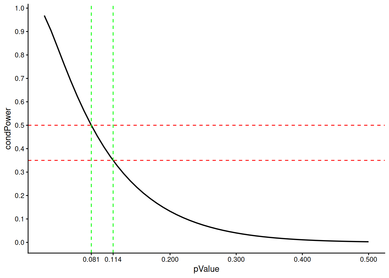
design |>
    getFutilityBounds(
        sourceValue = c(0.35, 0.5),
        sourceScale = "condPowerAtObserved",
        targetScale = "pValue"
    )
[1] 0.11398692 0.08101828As described above, we can now see that when the interim analysis is at \(t_1 = 0.5\) information rate (i.e. at half of the total information), a p-value boundary of approximately 0.081 corresponds to a conditional power at observed effect of 50%. If the conditional power threshold is lowered to 35%, the corresponding p-value boundary increases to approximately 0.114.
Predictive power vs. conditional power at observed effect
Here we illustrate how predictive power and conditional power at observed effect relate to each other. We select a design with no early efficacy stops and the interim at information rate 0.40:
design <- getDesignGroupSequential(
    typeOfDesign = "noEarlyEfficacy",
    alpha = 0.025,
    informationRates = c(0.4, 1)
)

futilityBounds <- seq(-0.5, 2.5, by = 0.025)

y <- design |>
    getFutilityBounds(
        sourceValue = futilityBounds,
        sourceScale = "zValue",
        targetScale = "predictivePower"
    )
dat <- data.frame(
    zValue = futilityBounds,
    CP = y,
    out = "pred"
)

y <- design |>
    getFutilityBounds(
        sourceValue = futilityBounds,
        sourceScale = "zValue",
        targetScale = "condPowerAtObserved"
    )
dat <- dat |> rbind(
    data.frame(
        zValue = futilityBounds,
        CP = y,
        out = "cond"
    )
)

dat |>
    ggplot(aes(zValue, CP, out)) +
        geom_line(aes(linetype = out), lwd = 0.75) +
        geom_hline(yintercept = 0.5, color = "red", lwd = 0.55) +
        theme_classic()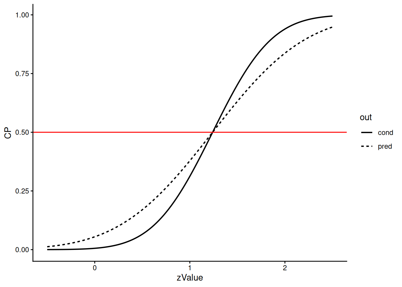
The Bayesian predictive power is always closer to 0.50 than the conditional power at observed effect and hence downweighs extreme results: For example, when the conditional power is only 1% then the predictive power is still 5%. The two power scales intersect at 50%, corresponding to a z-value of 1.170.
p-value vs. Bayesian predictive power/reverse conditional power
Both Bayesian predictive power/RCP and p-values are effect-size independent scales. Here we illustrate how they relate to each other for a design with no early efficacy stop at information rate = 0.5.
design <- getDesignGroupSequential(
    kMax = 2,
    typeOfDesign = "noEarlyEfficacy",
    alpha = 0.025
)

futilityBounds <- seq(0.1, 0.9, by = 0.01)
y <- design |>
    getFutilityBounds(
        sourceValue = futilityBounds,
        sourceScale = "pValue",
        targetScale = "predictivePower"
    )

data.frame(
    pValue = futilityBounds,
    predictivePower = y) |>
ggplot(aes(pValue, predictivePower)) +
    geom_line(lwd = 0.75) +
    geom_vline(
        xintercept = c(0.2, 0.4, 0.5),
        linetype = "dashed",
        color = "green",
        lwd = 0.5
    ) +
    geom_hline(
        yintercept = c(0.025, 0.055, 0.221),
        linetype = "dashed",
        color = "red",
        lwd = 0.5
    ) +
    scale_x_continuous(breaks = seq(0, 1, 0.1)) +
    scale_y_continuous(breaks = c(0, 0.025, 0.055, 0.1, 0.2, 0.221, 0.3, 0.4)) +
    theme_classic()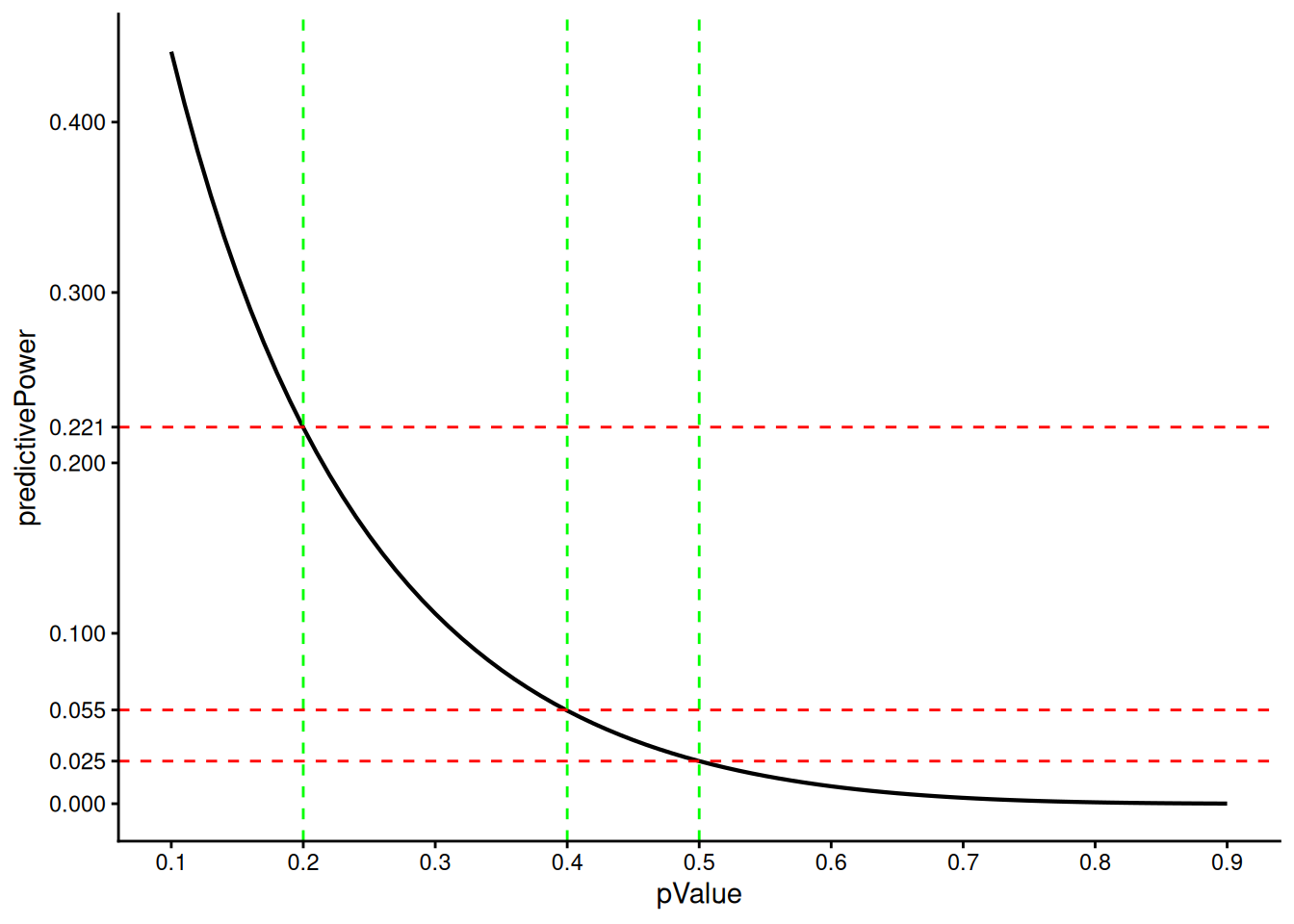
design |>
    getFutilityBounds(
        sourceValue = c(0.2, 0.4, 0.5),
        targetScale = "predictivePower",
        sourceScale = "pValue"

    )
[1] 0.22072949 0.05461352 0.02500000We see that a p-value of 0.5 corresponds to an Bayesian predictive power/RCP of 0.025, which was already mentioned above.
Remarks
The getFutilityBounds() function supports a summary() method that displays all information about the conversion:
getFutilityBounds(
    sourceValue = c(0.2, 0.4, 0.5),
    sourceScale = "pValue",
    targetScale = "zValue"
) |> summary()
Futility bounds summary:
User-defined parameters:
sourceValue: 0.2, 0.4, 0.5
sourceScale: 'pValue'
Default parameters:
targetScale: 'zValue'
Output:
targetValue: 0.842, 0.253, 0The functions getDesignGroupSequential(), getDesignInverseNormal(), and getDesignFisher() support the argument futilityBoundsScale which can be used to specify the scale of the futility bounds. The value must be one of zValue, pValue, reverseCondPower, condPowerAtObserved, or predictivePower. The default value is zValue for group-sequential and inverse normal designs and pValue for Fisher’s combination test designs.
Example
getDesignGroupSequential(
    typeOfDesign = "OF",
    alpha = 0.025,
    futilityBounds = c(0.5, 0.3),
    futilityBoundsScale = "pValue"
) |> summary()
Sequential analysis with a maximum of 3 looks (group sequential design)
O’Brien & Fleming design, non-binding futility, one-sided overall significance level 2.5%, power 80%, undefined endpoint, inflation factor 1.0668, ASN H1 0.849, ASN H01 0.842, ASN H0 0.6214.
| Stage | 1 | 2 | 3 |
|---|---|---|---|
| Planned information rate | 33.3% | 66.7% | 100% |
| Cumulative alpha spent | 0.0003 | 0.0072 | 0.0250 |
| Stage levels (one-sided) | 0.0003 | 0.0071 | 0.0225 |
| Efficacy boundary (z-value scale) | 3.471 | 2.454 | 2.004 |
| Futility boundary (z-value scale) | 0 | 0.524 | |
| Cumulative power | 0.0359 | 0.4635 | 0.8000 |
| Futility probabilities under H1 | 0.047 | 0.018 |
Summary
There are several complementary ways to define futility stopping in interim analyses. Depending on the design strategy and decision philosophy, futility may be based on classical test statistics, conditional or predictive quantities, or probability statements derived from the interim effect estimate.
Predictive interval plots offer an intuitive visual alternative. As discussed in Ortega-Villa et al. (2025), predictive intervals for future test statistics or effect estimates can be used to judge whether meaningful treatment effects remain plausible given the data observed so far. If the predictive interval lies almost entirely below the efficacy boundary, early stopping for futility becomes a natural conclusion.
A beta spending function provides yet another way to construct futility boundaries in a principled manner. Analogous to alpha spending for efficacy, beta spending distributes the Type II error budget across interim looks. This yields futility boundaries that are internally coherent, design-driven, and compatible with the desired overall power.
Importantly, all futility boundaries should be interpreted as guidelines rather than strict rules. They are typically implemented as non-binding rules, meaning that the sponsor or monitoring committee may decide to continue a trial even if a futility criterion is met, provided there is sufficient scientific or clinical justification to do so.
The getFutilityBounds() function in rpact is deliberately provided as a stand-alone tool to support this flexibility. It enables users to convert or reconstruct futility boundaries across multiple scales.
All transformations implemented in getFutilityBounds() have been extensively validated, including through reverse-transform checks ensuring that converting a boundary from one scale to another and back yields the same value within numerical tolerance.
Finally, the endpoint independent scales are implemented in the functions getDesignGroupSequential(), getDesignInverseNormal(), and getDesignFisher() using the argument futilityBoundsScale. This allows direct specification of futility boundaries on any endpoint independent scale when defining a design.
Endpoint dependent scales will be fully integrated into the sample size and power calculation functions of rpact in future releases.
References
Glimm, Ekkehard. 2012. “Comments on Adaptive Increase in Sample Size When Interim Results Are Promising: A Practical Guide with Examples by CR Mehta and SJ Pocock.” Statistics in Medicine 31 (1): 98–99.
Mehta, Cyrus R, and Stuart J Pocock. 2011. “Adaptive Increase in Sample Size When Interim Results Are Promising: A Practical Guide with Examples.” Statistics in Medicine 30 (28): 3267–84.
Ortega-Villa, Ana M, Megan C Grieco, Kevin Rubenstein, Jing Wang, and Michael A Proschan. 2025. “Futility Monitoring in Clinical Trials.” Statistics in Medicine 44 (13-14): e70157.
Tan, Ming, Xiaoping Xiong, and Michael H Kutner. 1998. “Clinical Trial Designs Based on Sequential Conditional Probability Ratio Tests and Reverse Stochastic Curtailing.” Biometrics, 682–95.
Wassmer, Gernot, and Werner Brannath. 2025. Group Sequential and Confirmatory Adaptive Designs in Clinical Trials. 2nd ed. Springer. https://link.springer.com/book/10.1007/978-3-031-89669-9.