library(rpact)
packageVersion("rpact") # version should be version 3.0 or laterDesigning Group Sequential Trials with Two Groups and a Continuous Endpoint with rpact
Planning
Means
This document provides examples for designing trials with continuous endpoints using rpact.
Introduction
These examples are not intended to replace the official rpact documentation and help pages but rather to supplement them. They also only cover a selection of all rpact features.
General convention: In rpact, arguments containing the index “2” always refer to the control group, “1” refer to the intervention group, and treatment effects compare treatment versus control.
First, load the rpact package
[1] '4.4.0.9305'Sample size calculation for a superiority trial without interim analyses
The sample size for a single-stage trial with continuous endpoints can be calculated using the function getSampleSizeMeans(). This function is fully documented in the relevant help page (?getSampleSizeMeans). Some examples are provided below.
getSampleSizeMeans() requires that the mean difference between the two arms is larger under the alternative than under the null hypothesis. For superiority trials, this implies that rpact requires that the targeted mean difference is >0 under the alternative hypothesis. If this is not the case, the function produces an error message. To circumvent this and power for a negative mean difference, one can simply switch the two arms (leading to a positive mean difference) as the situation is perfectly symmetric.
By default, getSampleSizeMeans() tests hypotheses about the mean difference. rpact also supports testing hypotheses about mean ratios if the argument meanRatio is set to TRUE but this will not be discussed further in this document.
By default, rpact uses sample size formulas for the \(t\)-test, i.e., it assumes that the standard deviation in the two groups is equal but unknown and estimated from the data. If sample size calculations for the \(z\)-test are desired, one can set the argument normalApproximation to TRUE but this is usually not recommended.
# Example of a standard trial:
# - targeted mean difference is 10 (alternative = 10)
# - standard deviation in both arms is assumed to be 24 (stDev = 24)
# - two-sided test (sided = 2), Type I error 0.05 (alpha = 0.05) and power 80%
# - (beta = 0.2)
sampleSizeResult <- getSampleSizeMeans(
    alternative = 10,
    stDev = 24,
    sided = 2,
    alpha = 0.05,
    beta = 0.2
)
sampleSizeResult
Design plan parameters and output for means
Design parameters
- Critical values: 1.960
- Two-sided power: FALSE
- Significance level: 0.0500
- Type II error rate: 0.2000
- Test: two-sided
User defined parameters
- Alternatives: 10
- Standard deviation: 24
Default parameters
- Mean ratio: FALSE
- Theta H0: 0
- Normal approximation: FALSE
- Treatment groups: 2
- Planned allocation ratio: 1
Sample size and output
- Number of subjects fixed: 182.8
- Number of subjects fixed (1): 91.4
- Number of subjects fixed (2): 91.4
- Lower critical values (treatment effect scale): -7.006
- Upper critical values (treatment effect scale): 7.006
Legend
- (i): values of treatment arm i
The generic summary() function produces the output
sampleSizeResult |> summary()Sample size calculation for a continuous endpoint
Fixed sample analysis, two-sided significance level 5%, power 80%. The results were calculated for a two-sample t-test, H0: mu(1) - mu(2) = 0, H1: effect = 10, standard deviation = 24.
| Stage | Fixed |
|---|---|
| Stage level (two-sided) | 0.0500 |
| Efficacy boundary (z-value scale) | 1.960 |
| Lower efficacy boundary (t) | -7.006 |
| Upper efficacy boundary (t) | 7.006 |
| Number of subjects | 182.8 |
Legend:
- (t): treatment effect scale
As per the output above, the required total sample size for the trial is 183 (184, when strictly adhering to equal group sizes) and the critical value corresponds to a minimal detectable mean difference of approximately 7.01.
Unequal randomization between the treatment groups can be defind with allocationRatioPlanned, for example,
# Extension of standard trial:
# - 2(intervention):1(control) randomization (allocationRatioPlanned = 2)
getSampleSizeMeans(
    alternative = 10,
    stDev = 24,
    allocationRatioPlanned = 2,
    sided = 2,
    alpha = 0.05,
    beta = 0.2
) |>
  summary()
Sample size calculation for a continuous endpoint
Fixed sample analysis, two-sided significance level 5%, power 80%. The results were calculated for a two-sample t-test, H0: mu(1) - mu(2) = 0, H1: effect = 10, standard deviation = 24, planned allocation ratio = 2.
| Stage | Fixed |
|---|---|
| Stage level (two-sided) | 0.0500 |
| Efficacy boundary (z-value scale) | 1.960 |
| Lower efficacy boundary (t) | -7.004 |
| Upper efficacy boundary (t) | 7.004 |
| Number of subjects | 205.4 |
Legend:
- (t): treatment effect scale
Power for a given sample size can be calculated using the function getPowerMeans() which has the same arguments as getSampleSizeMeans() except that the maximum total sample is given (maxNumberOfSubjects) instead of the Type II error (beta).
# Calculate power for the 2:1 randomized trial with total sample size 206
# (as above) assuming a larger difference of 12
powerResult <- getPowerMeans(
    alternative = 12,
    stDev = 24,
    sided = 2,
    allocationRatioPlanned = 2,
    maxNumberOfSubjects = 206,
    alpha = 0.05
)
powerResult
Design plan parameters and output for means
Design parameters
- Critical values: 1.960
- Significance level: 0.0500
- Test: two-sided
User defined parameters
- Alternatives: 12
- Standard deviation: 24, 24
- Planned allocation ratio: 2
- Direction upper: NA
- Maximum number of subjects: 206
Default parameters
- Mean ratio: FALSE
- Theta H0: 0
- Normal approximation: FALSE
- Treatment groups: 2
Power and output
- Effect: 12
- Overall reject: 0.9203
- Number of subjects fixed: 206
- Number of subjects fixed (1): 137.3
- Number of subjects fixed (2): 68.7
- Lower critical values (treatment effect scale): -6.994
- Upper critical values (treatment effect scale): 6.994
Legend
- (i): values of treatment arm i
The calculated power is provided in the output as “Overall reject” and is 0.92 for the example alternative = 12.
The summary() function produces
powerResult |> summary()Power calculation for a continuous endpoint
Fixed sample analysis, two-sided significance level 5%. The results were calculated for a two-sample t-test, H0: mu(1) - mu(2) = 0, H1: effect = 12, standard deviation = 24, number of subjects = 206, planned allocation ratio = 2.
| Stage | Fixed |
|---|---|
| Stage level (two-sided) | 0.0500 |
| Efficacy boundary (z-value scale) | 1.960 |
| Lower efficacy boundary (t) | -6.994 |
| Upper efficacy boundary (t) | 6.994 |
| Power | 0.9203 |
| Number of subjects | 206.0 |
Legend:
- (t): treatment effect scale
getPowerMeans() (as well as getSampleSizeMeans()) can also be called with a vector argument for the mean difference under the alternative H1 (alternative). This is illustrated below via a plot of power depending on these values. For examples of all available plots, see the R Markdown document How to create admirable plots with rpact.
# Example: Calculate power for design with sample size 206 as above
# alternative values ranging from 5 to 15
powerResult <- getPowerMeans(
    alternative = 5:15,
    stDev = 24,
    sided = 2,
    allocationRatioPlanned = 2,
    maxNumberOfSubjects = 206,
    alpha = 0.05
)
powerResult |> plot(type = 7) # one of several possible plots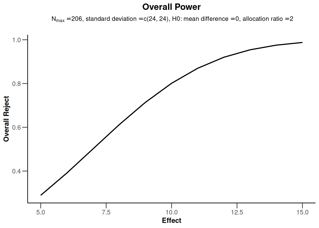
Sample size calculation for a non-inferiority trial without interim analyses
The sample size calculation proceeds in the same fashion as for superiority trials except that the role of the null and the alternative hypothesis are reversed and the test is always one-sided. In this case, the non-inferiority margin \(\Delta\) corresponds to the treatment effect under the null hypothesis (thetaH0) which one aims to reject.
# Example: Non-inferiority trial with margin delta = 12, standard deviation = 14
# - One-sided alpha = 0.05, 1:1 randomization
# - H0: treatment difference <= -12 (i.e., = -12 for calculations, thetaH0 = -12)
#    vs. alternative H1: treatment difference = 0 (alternative = 0)
getSampleSizeMeans(
    thetaH0 = -12,
    alternative = 0,
    stDev = 14,
    alpha = 0.025,
    beta = 0.2,
    sided = 1
) |>
  print()
Design plan parameters and output for means
Design parameters
- Critical values: 1.960
- Significance level: 0.0250
- Type II error rate: 0.2000
- Test: one-sided
User defined parameters
- Theta H0: -12
- Alternatives: 0
- Standard deviation: 14
Default parameters
- Mean ratio: FALSE
- Normal approximation: FALSE
- Treatment groups: 2
- Planned allocation ratio: 1
Sample size and output
- Number of subjects fixed: 44.7
- Number of subjects fixed (1): 22.4
- Number of subjects fixed (2): 22.4
- Critical values (treatment effect scale): -3.556
Legend
- (i): values of treatment arm i
Sample size calculation for group sequential designs
Sample size calculation for a group sequential trials is performed in two steps:
- Define the (abstract) group sequential design using the function
getDesignGroupSequential(). For details regarding this step, see the R markdown file Defining group sequential boundaries with rpact. - Calculate sample size for the continuous endpoint by feeding the abstract design into the function
getSampleSizeMeans().
In general, rpact supports both one-sided and two-sided group sequential designs. However, if futility boundaries are specified, only one-sided tests are permitted. For simplicity, it is often preferred to use one-sided tests for group sequential designs (typically, with \(\alpha = 0.025\)).
R code for a simple example is provided below:
# Example: Group-sequential design with  O'Brien & Fleming type alpha-spending
# and one interim at 60% information
design <- getDesignGroupSequential(
    sided = 1,
    alpha = 0.025,
    beta = 0.2,
    informationRates = c(0.6, 1),
    typeOfDesign = "asOF"
)

# Trial assumes an effect size of 10 as above, a stDev = 24, and an allocation
# ratio of 2
sampleSizeResultGS <- getSampleSizeMeans(
    design,
    alternative = 10,
    stDev = 24,
    allocationRatioPlanned = 2
)
# Standard rpact output (sample size object only, not design object)
sampleSizeResultGS
Design plan parameters and output for means
Design parameters
- Information rates: 0.600, 1.000
- Critical values: 2.669, 1.981
- Futility bounds (non-binding): -Inf
- Cumulative alpha spending: 0.003808, 0.025000
- Local one-sided significance levels: 0.003808, 0.023798
- Significance level: 0.0250
- Type II error rate: 0.2000
- Test: one-sided
User defined parameters
- Alternatives: 10
- Standard deviation: 24
- Planned allocation ratio: 2
Default parameters
- Mean ratio: FALSE
- Theta H0: 0
- Normal approximation: FALSE
- Treatment groups: 2
Sample size and output
- Maximum number of subjects: 207.1
- Maximum number of subjects (1): 138.1
- Maximum number of subjects (2): 69
- Number of subjects [1]: 124.3
- Number of subjects [2]: 207.1
- Number of subjects (1) [1]: 82.9
- Number of subjects (1) [2]: 138.1
- Number of subjects (2) [1]: 41.4
- Number of subjects (2) [2]: 69
- Reject per stage [1]: 0.3123
- Reject per stage [2]: 0.4877
- Early stop: 0.3123
- Expected number of subjects under H0: 206.8
- Expected number of subjects under H0/H1: 202.4
- Expected number of subjects under H1: 181.3
- Critical values (treatment effect scale) [1]: 12.393
- Critical values (treatment effect scale) [2]: 7.050
Legend
- (i): values of treatment arm i
- [k]: values at stage k
# Summary rpact output for sample size object
sampleSizeResultGS |> summary()
Sample size calculation for a continuous endpoint
Sequential analysis with a maximum of 2 looks (group sequential design), one-sided overall significance level 2.5%, power 80%. The results were calculated for a two-sample t-test, H0: mu(1) - mu(2) = 0, H1: effect = 10, standard deviation = 24, planned allocation ratio = 2.
| Stage | 1 | 2 |
|---|---|---|
| Planned information rate | 60% | 100% |
| Cumulative alpha spent | 0.0038 | 0.0250 |
| Stage levels (one-sided) | 0.0038 | 0.0238 |
| Efficacy boundary (z-value scale) | 2.669 | 1.981 |
| Efficacy boundary (t) | 12.393 | 7.050 |
| Cumulative power | 0.3123 | 0.8000 |
| Number of subjects | 124.3 | 207.1 |
| Expected number of subjects under H1 | 181.3 | |
| Exit probability for efficacy (under H0) | 0.0038 | |
| Exit probability for efficacy (under H1) | 0.3123 |
Legend:
- (t): treatment effect scale
System: rpact 4.4.0.9305, R version 4.6.0 (2026-04-24), platform: x86_64-pc-linux-gnu
To cite R in publications use:
R Core Team (2026). R: A Language and Environment for Statistical Computing. R Foundation for Statistical Computing, Vienna, Austria. doi:10.32614/R.manuals https://doi.org/10.32614/R.manuals. https://www.R-project.org/.
To cite package ‘rpact’ in publications use:
Wassmer G, Pahlke F (2026). rpact: Confirmatory Adaptive Clinical Trial Design and Analysis. R package version 4.4.0.9305. doi:10.32614/CRAN.package.rpact
Wassmer G, Brannath W (2025). Group Sequential and Confirmatory Adaptive Designs in Clinical Trials, 2nd edition. Springer, Cham, Switzerland. ISBN 978-3-031-89668-2. doi:10.1007/978-3-031-89669-9 https://doi.org/10.1007/978-3-031-89669-9.