How to Create One- and Multi-Arm Analysis Result Plots with rpact

Utilities

This document provides different examples for creating one- and multi-arm analysis result plots with rpact and ggplot2.

Author

Published

November 6, 2025

Preparation

First, load the rpact package

library(rpact)
packageVersion("rpact") # version should be version 3.0 or later

[1] '4.3.0.9292'

Create a design

designIN <- getDesignInverseNormal(
    kMax = 4, alpha = 0.02,
    futilityBounds = c(-0.5, 0, 0.5), 
    bindingFutility = FALSE,
    typeOfDesign = "asKD", 
    gammaA = 1.2,
    informationRates = c(0.15, 0.4, 0.7, 1)
)

designF <- getDesignFisher(
    kMax = 4, 
    alpha = 0.02,
    informationRates = c(0.15, 0.4, 0.7, 1)
)

Analysis results base

Analysis results base - means

simpleDataExampleMeans1 <- getDataset(
    n = c(120, 130, 130),
    means = c(0.45, 0.51, 0.45) * 100,
    stDevs = c(1.3, 1.4, 1.2) * 100
)

x <- getAnalysisResults(
    design = designIN, 
    dataInput = simpleDataExampleMeans1,
    nPlanned = 130, 
    thetaH0 = 30, 
    thetaH1 = 60, 
    assumedStDev = 100
)

Calculation of final confidence interval performed for kMax = 4 (for kMax > 2, it is theoretically shown that it is valid only if no sample size change was performed)

plot(x, thetaRange = c(10, 80))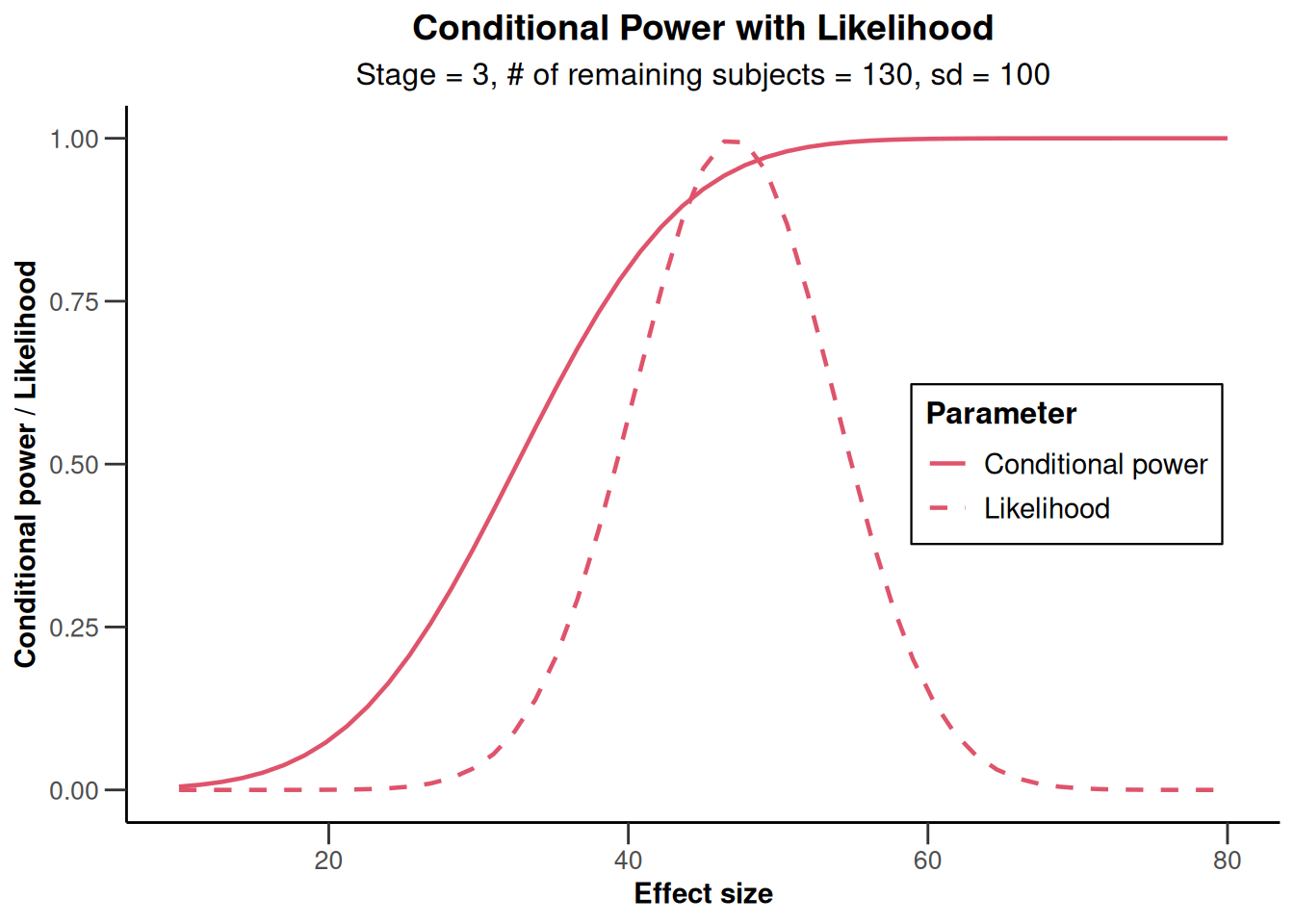

NULL

plot(x, type = 2)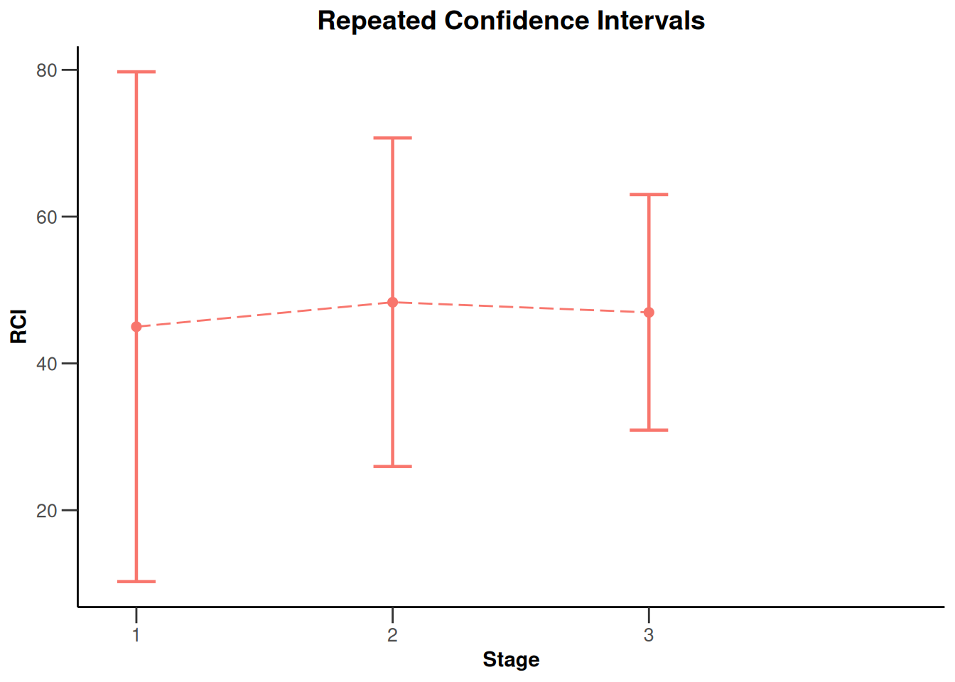

simpleDataExampleMeans2 <- getDataset(
    n1 = c(23, 13, 22, 13),
    n2 = c(22, 11, 22, 11),
    means1 = c(2.7, 2.5, 4.5, 2.5) * 100,
    means2 = c(1, 1.1, 1.3, 1) * 100,
    stds1 = c(1.3, 2.4, 2.2, 1.3) * 100,
    stds2 = c(1.2, 2.2, 2.1, 1.3) * 100
)

x <- getAnalysisResults(
    design = designIN, 
    dataInput = simpleDataExampleMeans2,
    thetaH0 = 110, 
    equalVariances = TRUE, 
    directionUpper = TRUE, 
    stage = 2
)
x |> plot(nPlanned = c(20, 30))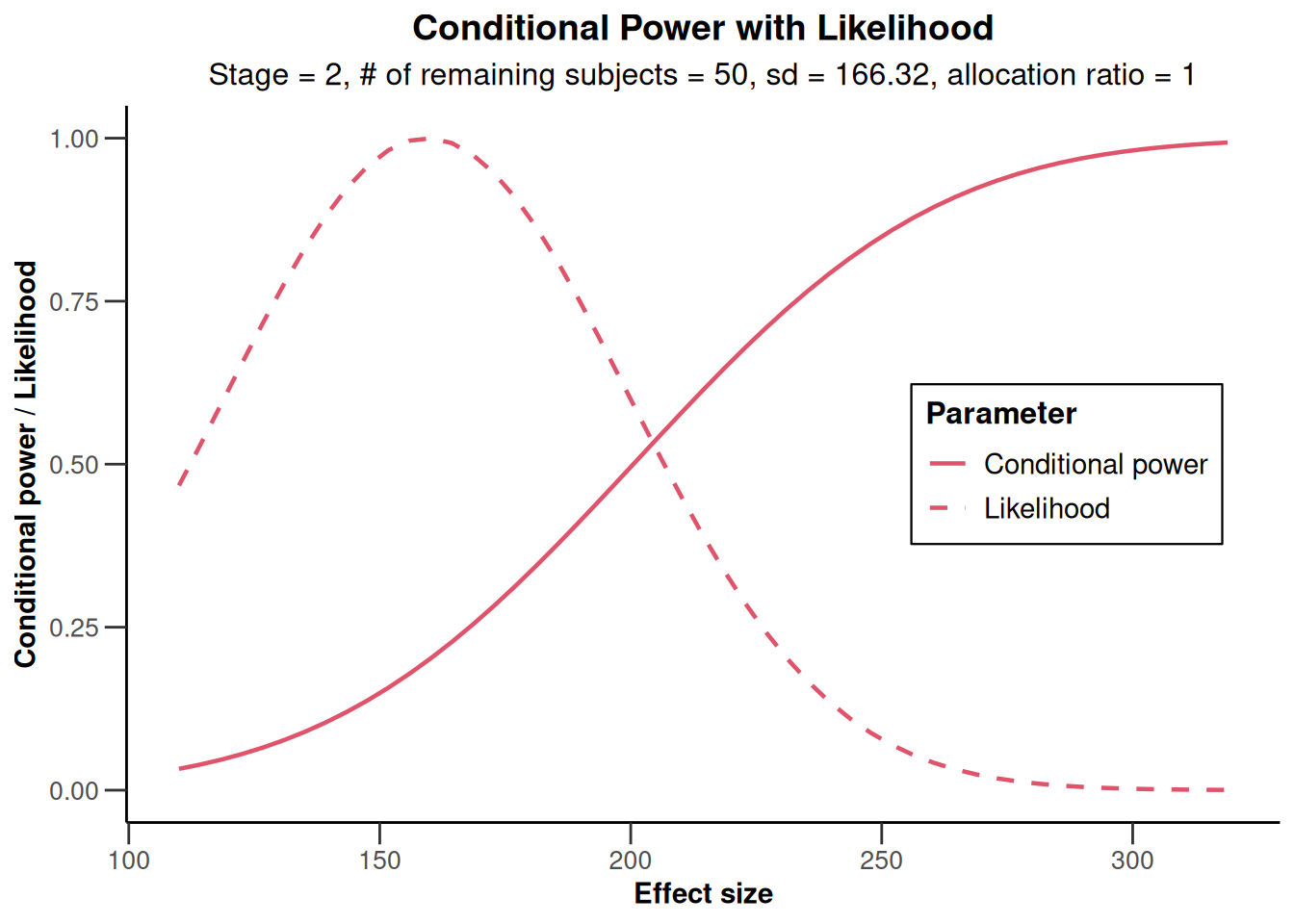

NULL

x |> plot(type = 2)

Analysis results base - rates

simpleDataExampleRates1 <- getDataset(
    n = c(8, 10, 9, 11),
    events = c(4, 5, 5, 6)
)

x <- getAnalysisResults(
    design = designIN, 
    dataInput = simpleDataExampleRates1,
    stage = 3, 
    thetaH0 = 0.75, 
    normalApproximation = TRUE,
    directionUpper = FALSE, 
    nPlanned = 10
)

Calculation of final confidence interval performed for kMax = 4 (for kMax > 2, it is theoretically shown that it is valid only if no sample size change was performed)

x |> plot()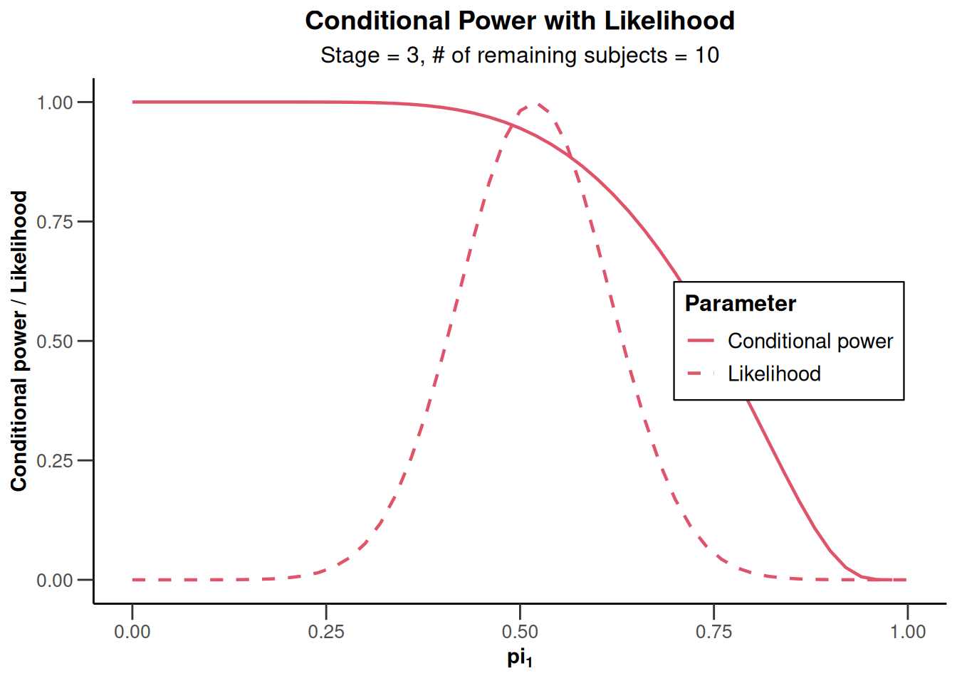

NULL

x |> plot(type = 2)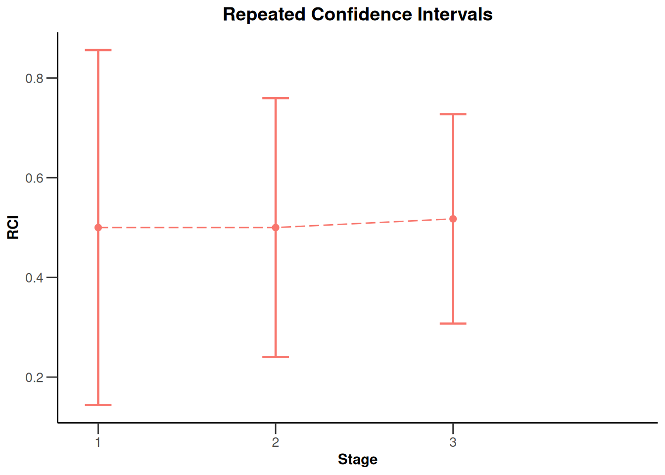

x <- getAnalysisResults(
    design = designIN, 
    dataInput = simpleDataExampleRates1,
    stage = 3, 
    thetaH0 = 0.75, 
    normalApproximation = FALSE,
    directionUpper = FALSE
)
x |> plot(nPlanned = 20)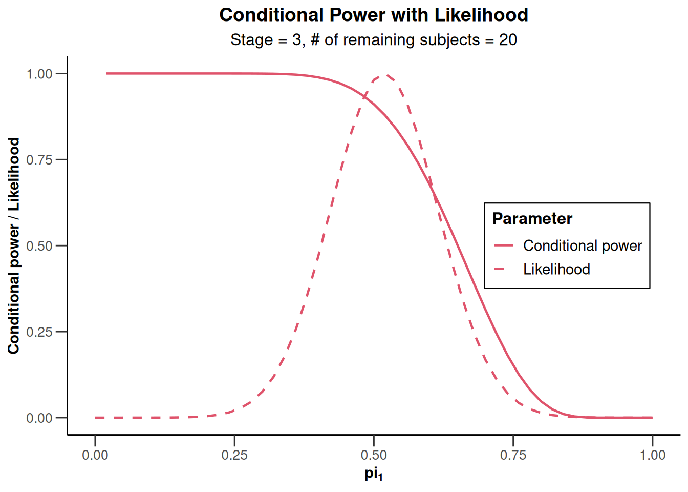

NULL

x |> plot(type = 2)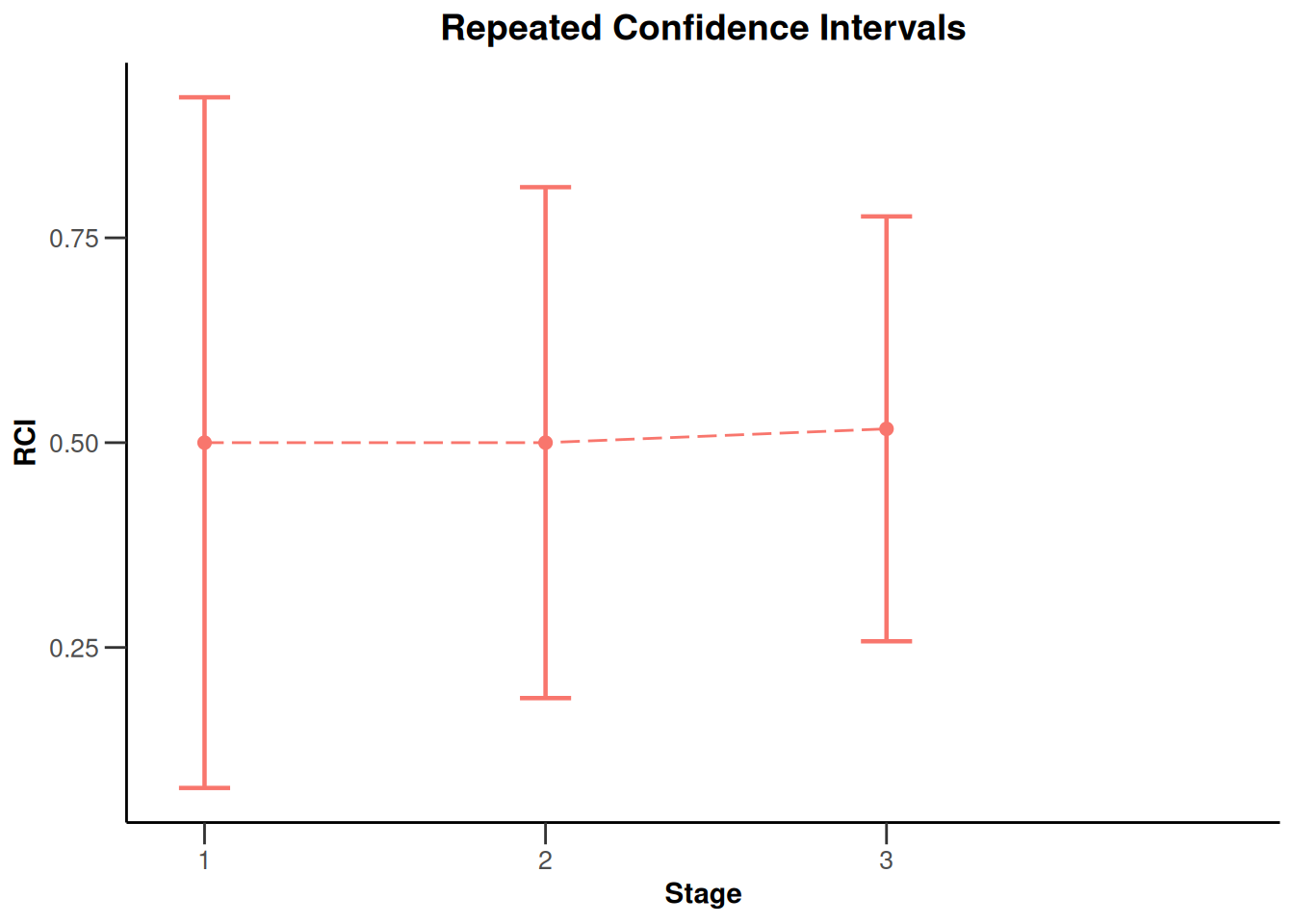

simpleDataExampleRates2 <- getDataset(
    n1 = c(17, 23, 22),
    n2 = c(18, 20, 19),
    events1 = c(11, 12, 17),
    events2 = c(5, 10, 7)
)

x <- getAnalysisResults(
  designIN, simpleDataExampleRates2,
  thetaH0 = 0,
  stage = 2, 
  directionUpper = TRUE, 
  normalApproximation = FALSE,
  pi1 = 0.9, 
  pi2 = 0.3, 
  nPlanned = c(20, 20)
)

Repeated confidence intervals will be calculated under the normal approximation

x |> plot(piTreatmentRange = c(0.2, 0.8))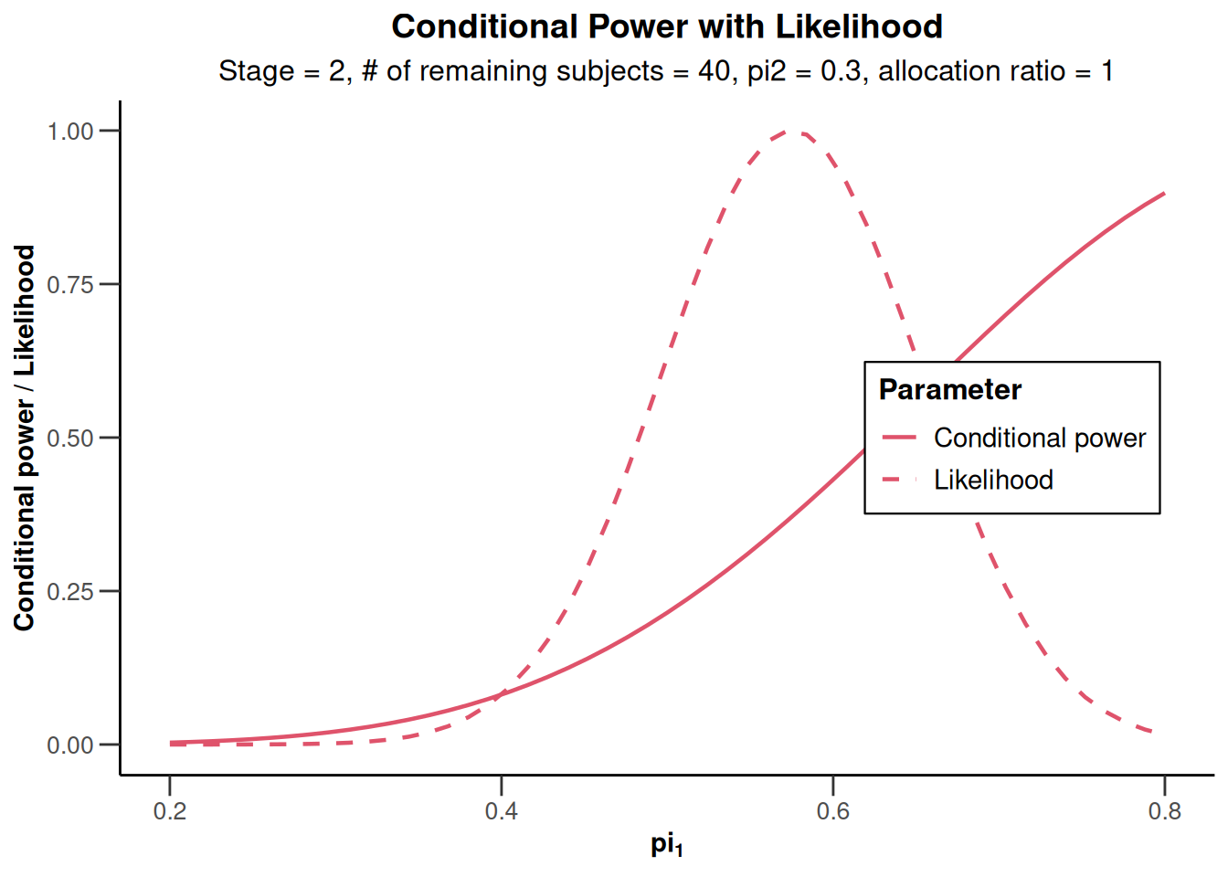

NULL

x |> plot(type = 2)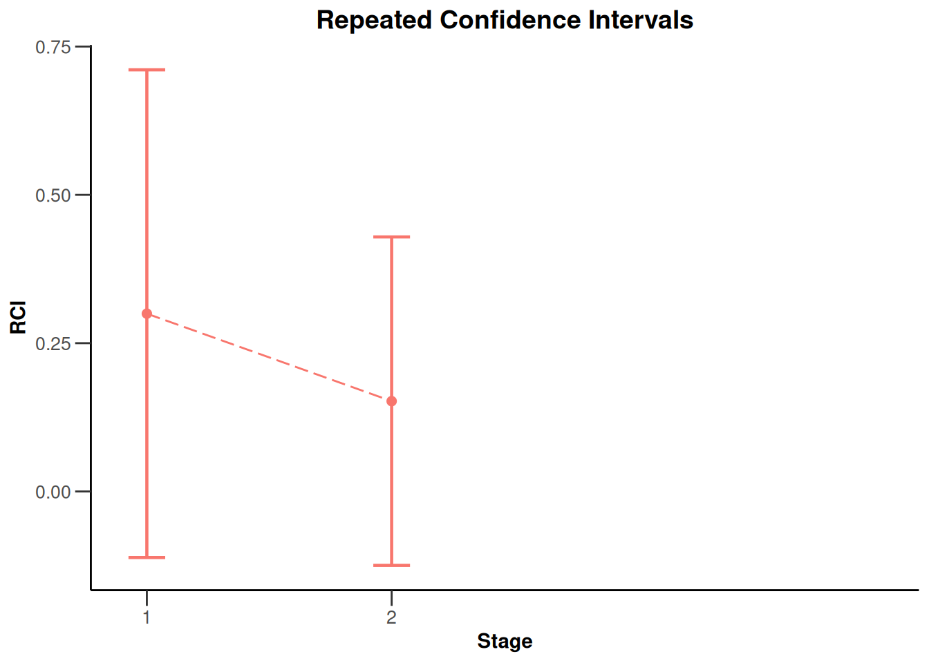

Analysis results base - survival

simpleDataExampleSurvival <- getDataset(
    overallEvents = c(8, 15, 29),
    overallAllocationRatios = c(1, 1, 1),
    overallLogRanks = c(1.52, 1.38, 2.9)
)

x <- getAnalysisResults(designIN,
    simpleDataExampleSurvival,
    directionUpper = TRUE, 
    nPlanned = 20
)

Calculation of final confidence interval performed for kMax = 4 (for kMax > 2, it is theoretically shown that it is valid only if no sample size change was performed)

x |> plot(thetaRange = c(1, 3))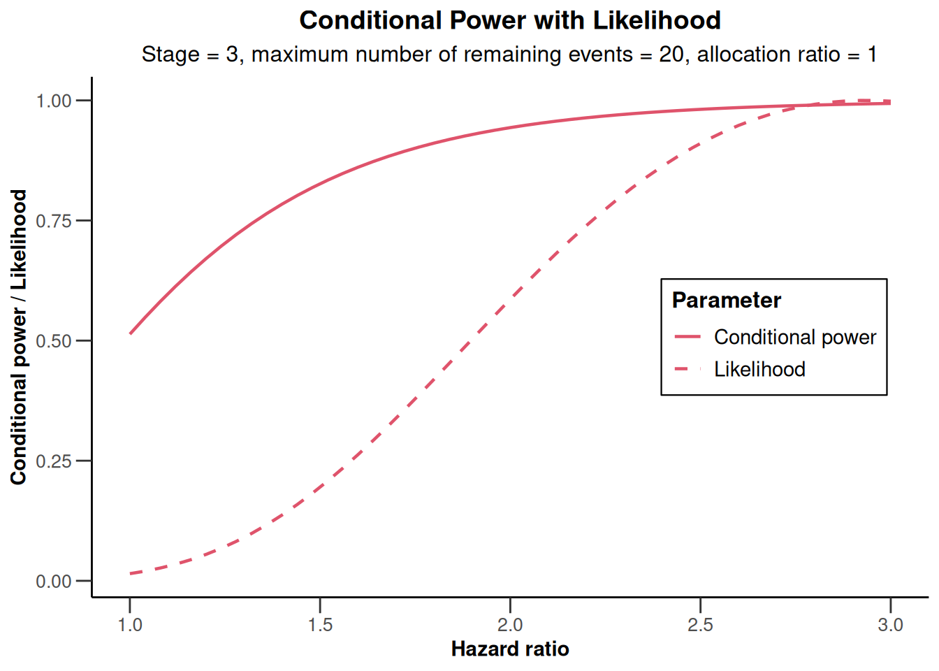

NULL

x |> plot(type = 2)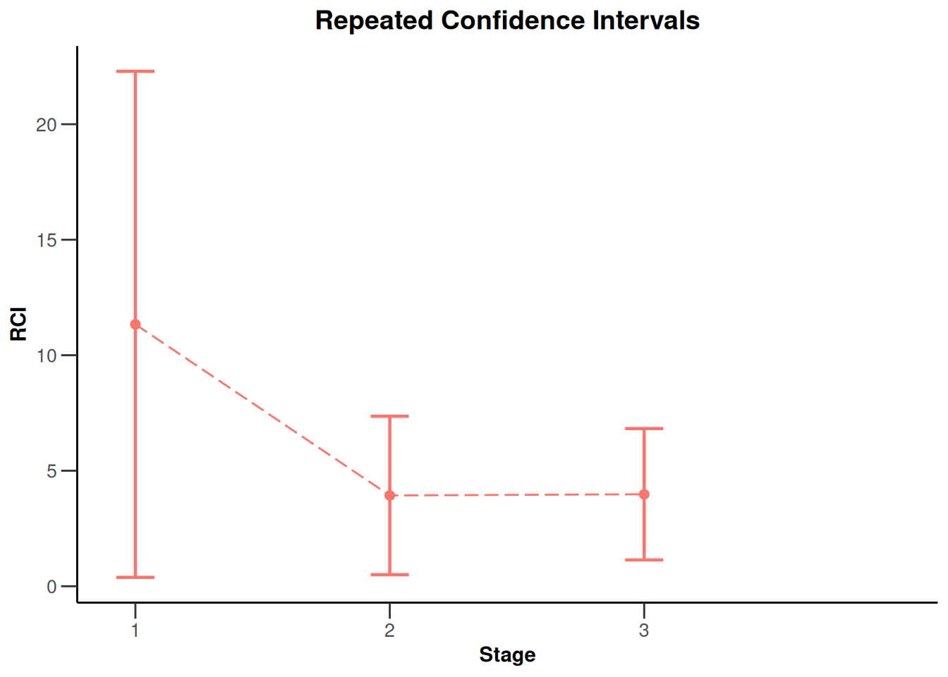

Analysis results multi-arm

Analysis results multi-arm - means

dataExampleMeans <- getDataset(
    n1 = c(13, 25),
    n2 = c(15, NA),
    n3 = c(14, 27),
    n4 = c(12, 29),
    means1 = c(242, 222),
    means2 = c(188, NA),
    means3 = c(267, 277),
    means4 = c(92, 122),
    stDevs1 = c(244, 221),
    stDevs2 = c(212, NA),
    stDevs3 = c(256, 232),
    stDevs4 = c(215, 227)
)

x <- getAnalysisResults(
    design = designF, 
    dataInput = dataExampleMeans,
    intersectionTest = "Simes", 
    directionUpper = TRUE,
    varianceOption = "notPooled", 
    nPlanned = c(32, 8),
    assumedStDevs = c(200, NA, 240)
)

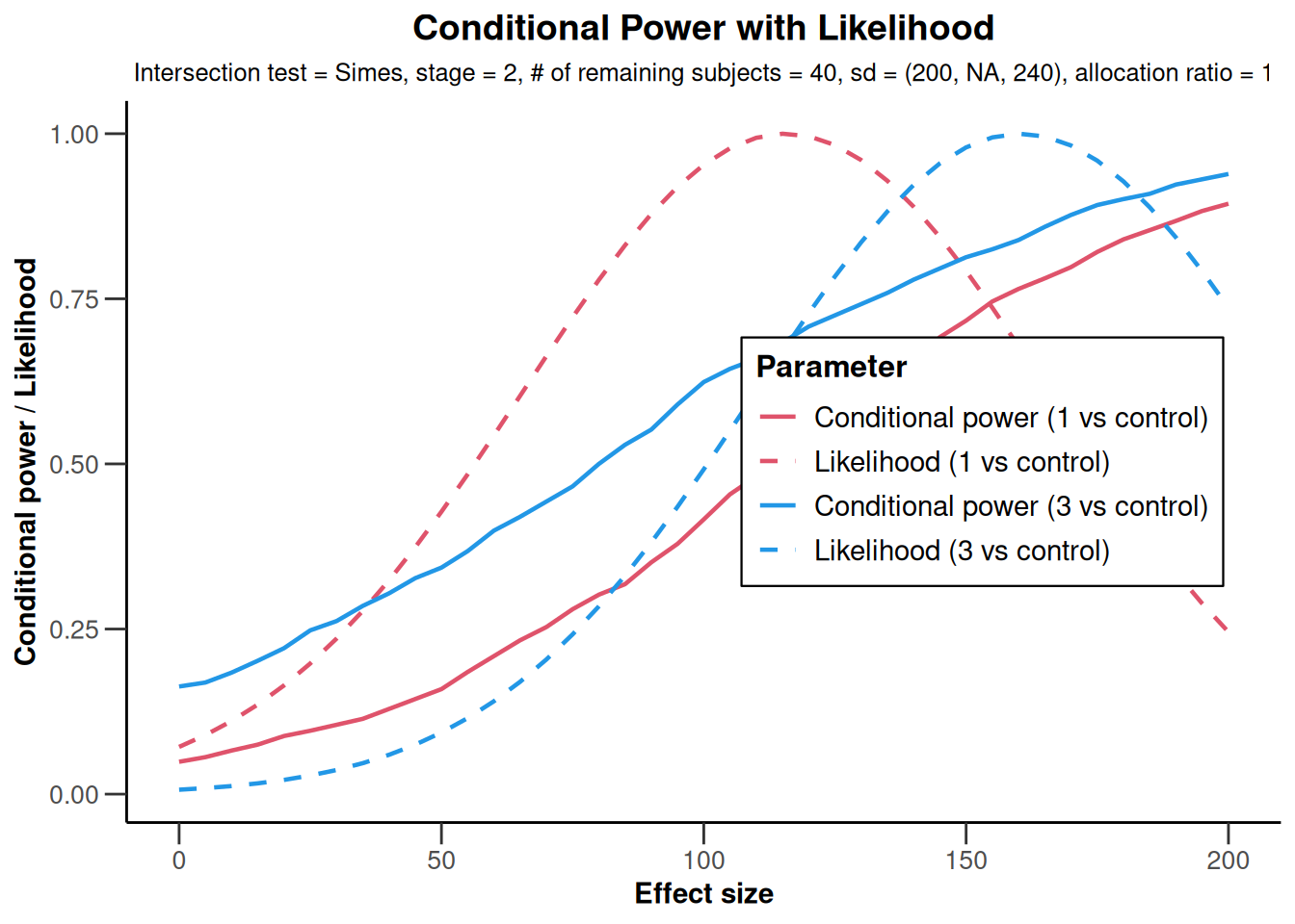
x |> plot()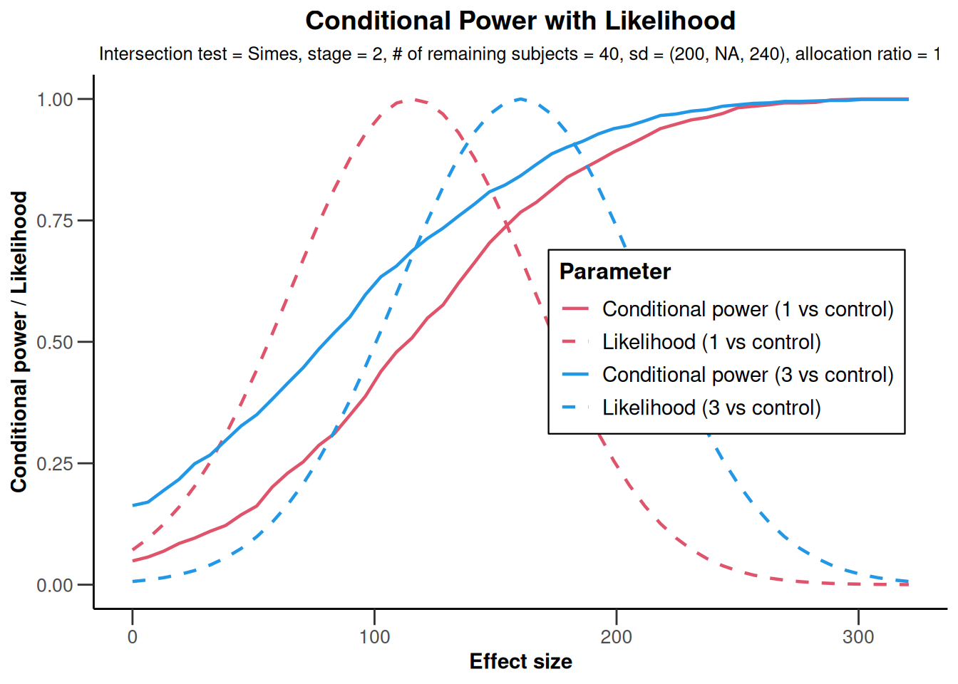

NULL

x |> plot(
    nPlanned = c(32, 8), 
    thetaRange = seq(0, 200, 5),
    assumedStDevs = c(200, NA, 240), 
    treatmentArms = c(1, 3)
)

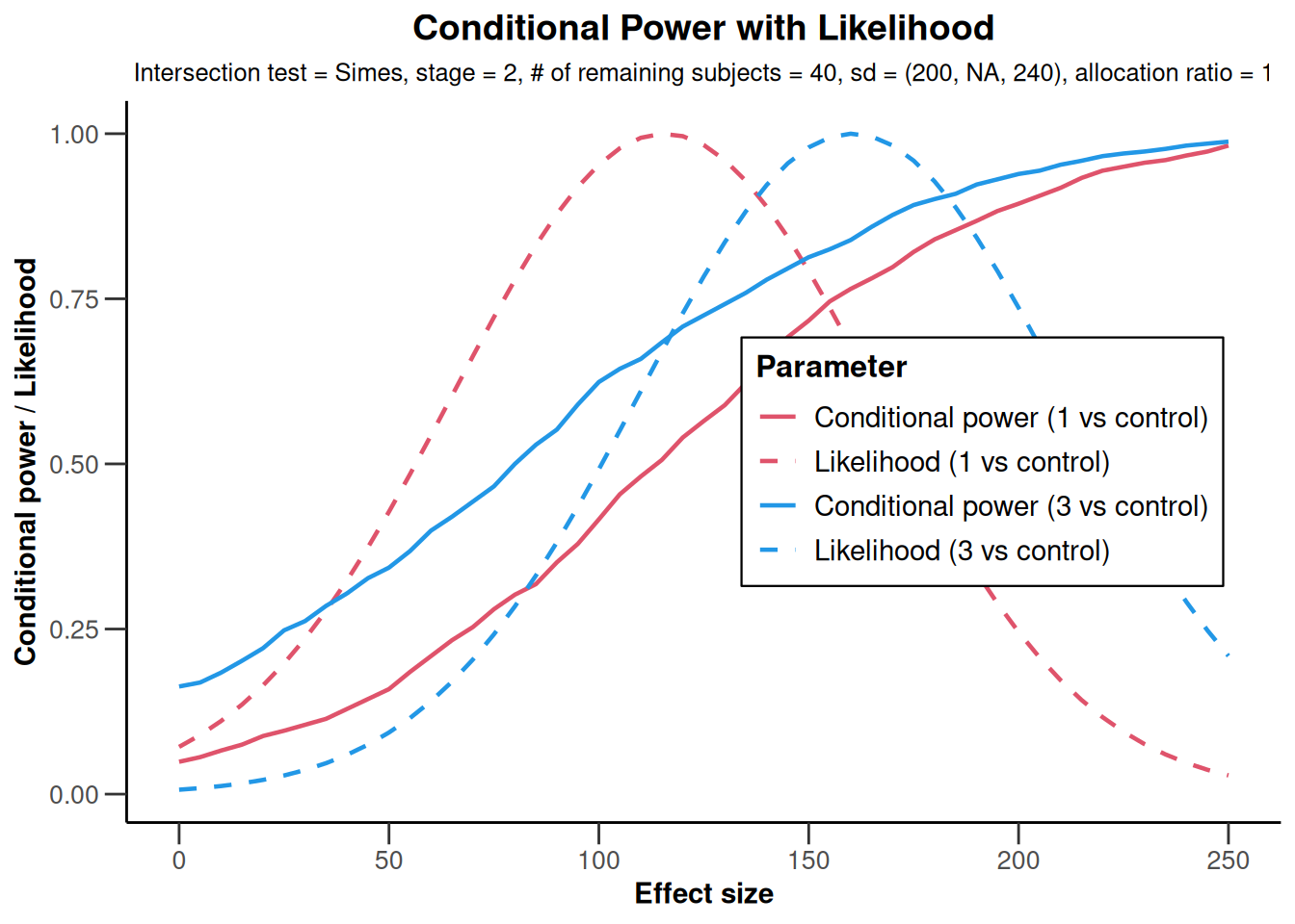
NULL

x |> plot(
    nPlanned = c(32, 8), 
    thetaRange = c(0, 250),
    assumedStDevs = c(200, NA, 240), 
    treatmentArms = c(1, 3)
)

NULL

x |> plot(type = 2)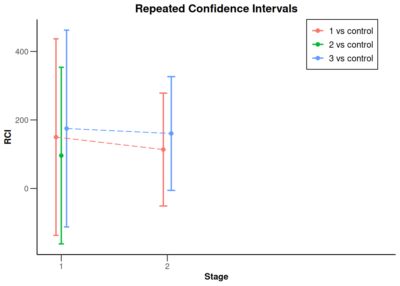

x |> plot(type = 2, treatmentArms = c(1, 3))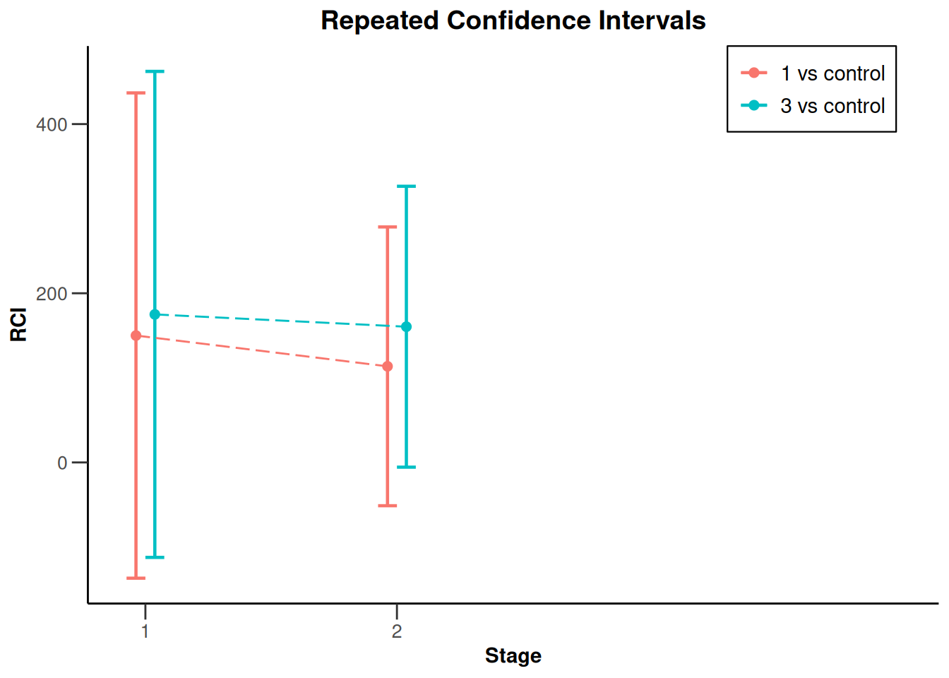

x |> plot(type = 2, treatmentArms = c(1))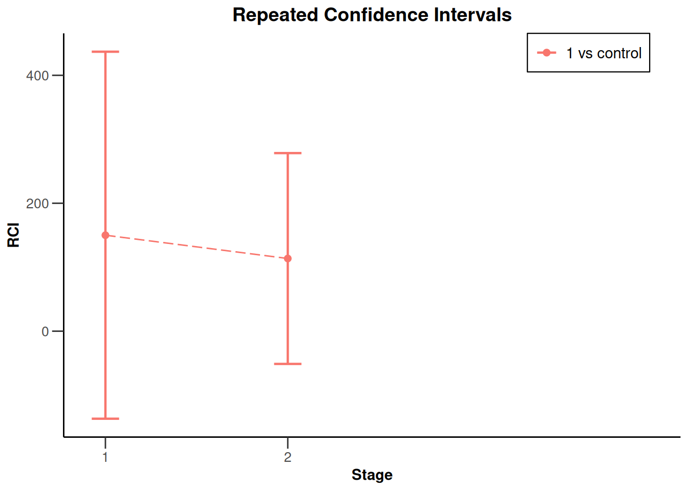

x |> plot(type = 2, treatmentArms = c(2))

`geom_line()`: Each group consists of only one observation.
ℹ Do you need to adjust the group aesthetic?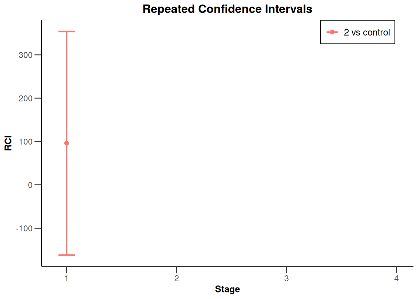

x |> plot(type = 2, treatmentArms = c(3))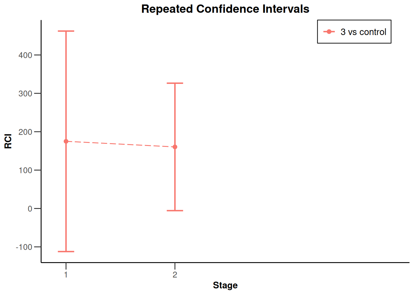

x2 <- getAnalysisResults(
    design = designIN, 
    dataInput = dataExampleMeans,
    intersectionTest = "Simes", 
    directionUpper = TRUE,
    varianceOption = "notPooled", 
    nPlanned = c(32, 8)
)
# Observed standard deviations will be used
x2 |> plot()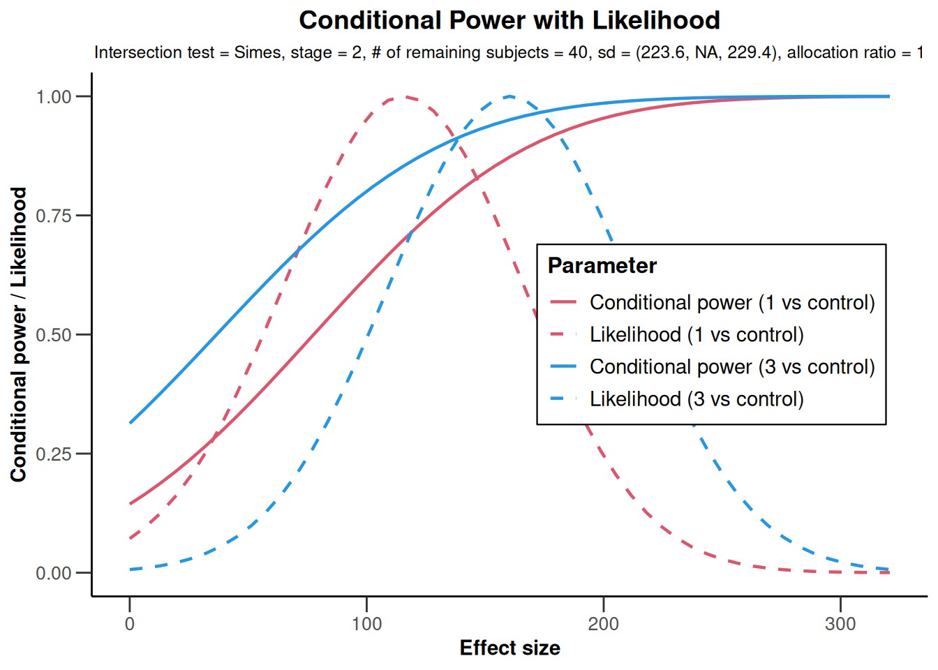

NULL

Analysis results multi-arm - rates

dataExampleRates <- getDataset(
    n1 = c(23, 25),
    n2 = c(25, NA),
    n3 = c(24, 27),
    n4 = c(22, 29),
    events1 = c(15, 12),
    events2 = c(19, NA),
    events3 = c(18, 22),
    events4 = c(12, 13)
)

analysisResultsRates <- getAnalysisResults(
    design = designIN,
    dataInput = dataExampleRates, 
    intersectionTest = "Simes",
    nPlanned = c(20, 20), 
    directionUpper = TRUE, 
    piControl = 0.2
)

analysisResultsRates |> plot()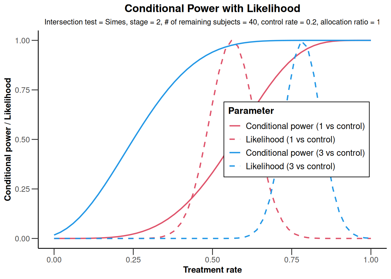

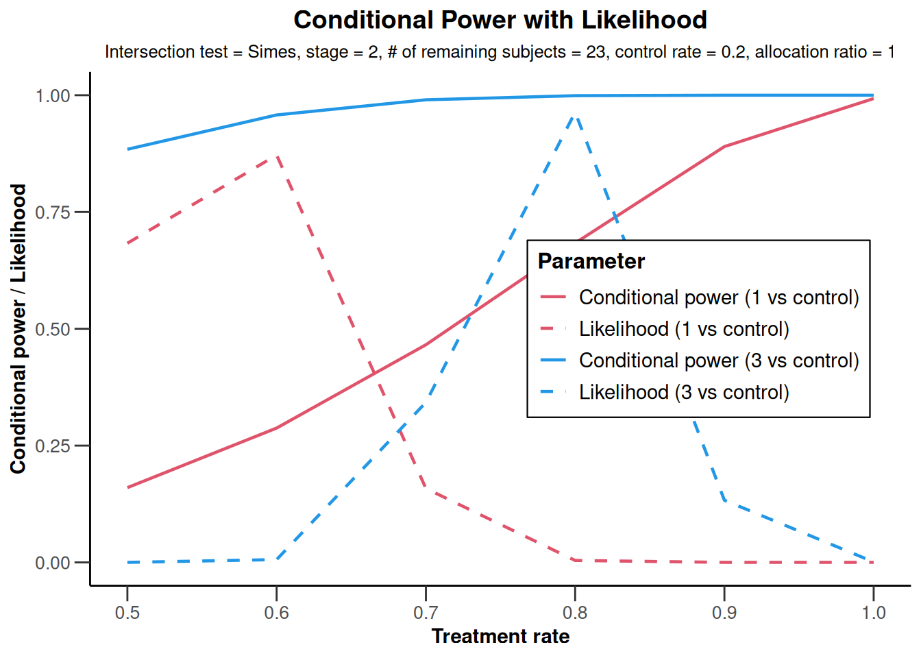
NULL

analysisResultsRates |> 
  plot(
    nPlanned = c(20, 3),
    piTreatmentRange = seq(0.5, 1, 0.1)
)

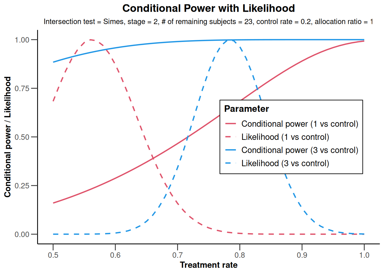
NULL

analysisResultsRates |> 
  plot(
    nPlanned = c(20, 3),
    piTreatmentRange = c(0.5, 1)
)

NULL

analysisResultsRates |> 
  plot(nPlanned = c(20, 3))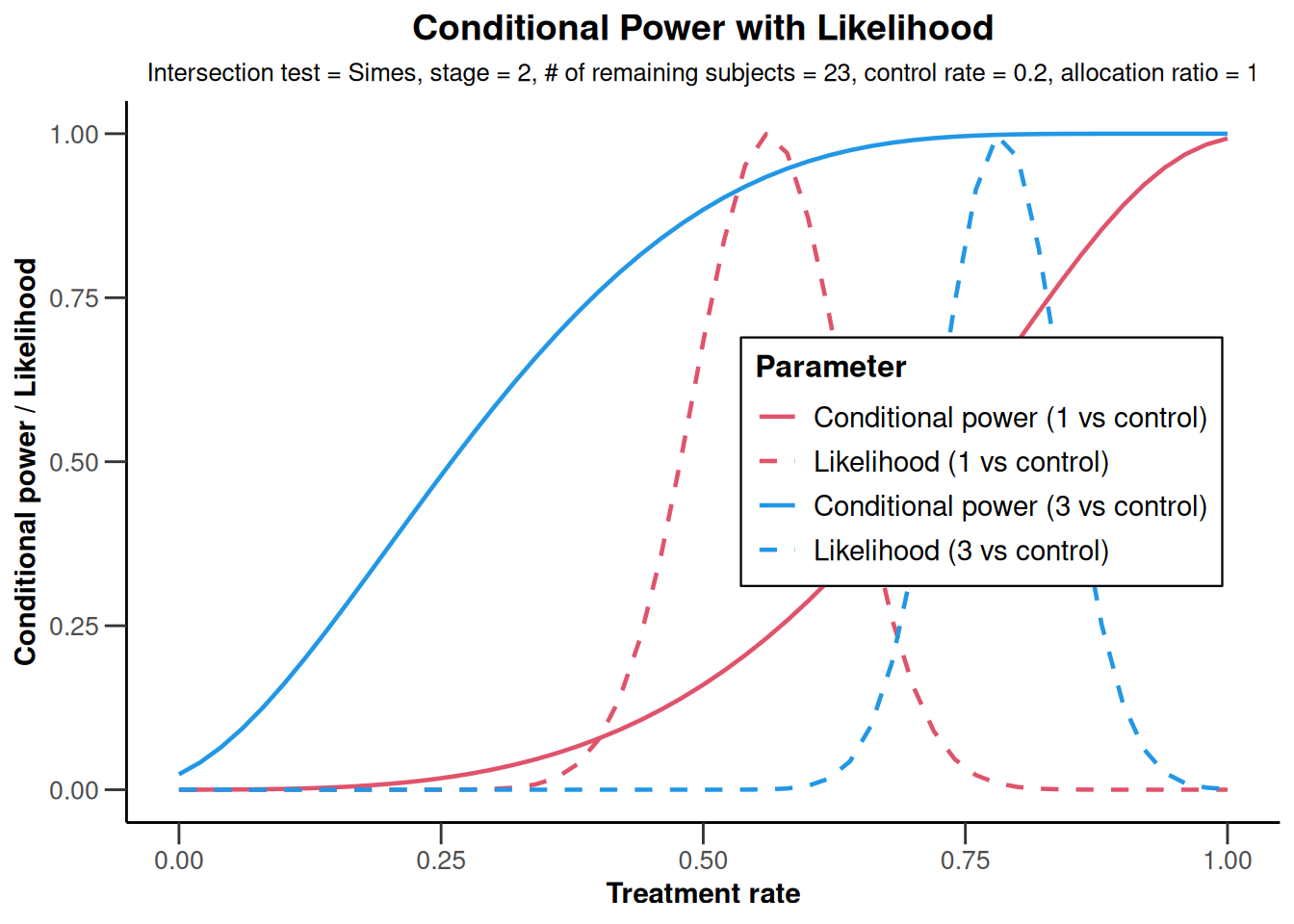

NULL

analysisResultsRates |>
  plot(type = 2)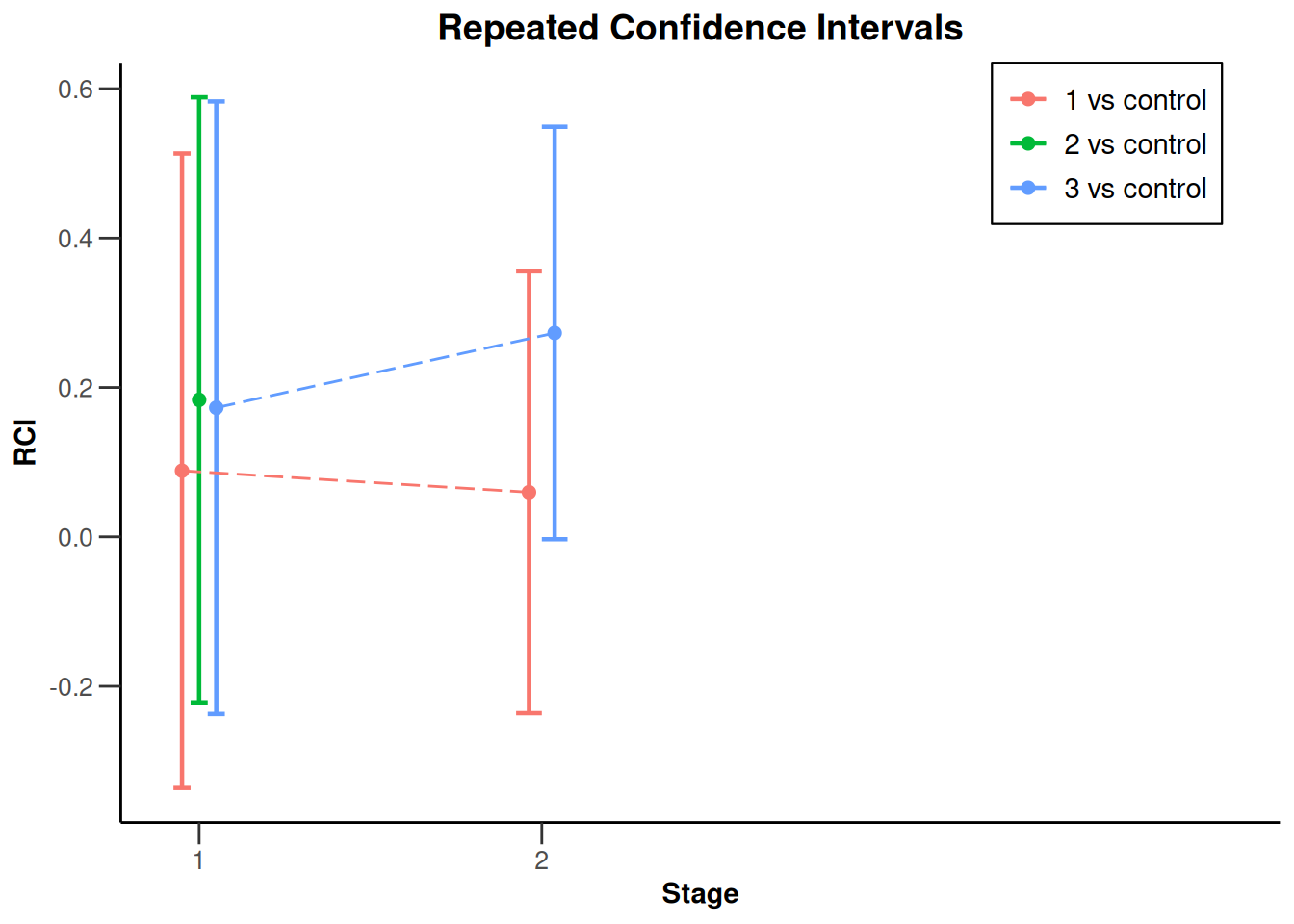

Analysis results multi-arm - survival

dataExampleSurvival <- getDataset(
    events1 = c(25, 32),
    events2 = c(18, NA),
    events3 = c(22, 36),
    logRanks1 = c(1.9, 1.8),
    logRanks2 = c(1.99, NA),
    logRanks3 = c(2.52, 2.11)
)

analysisResultsSurvival <- getAnalysisResults(
    design = getDesignInverseNormal(),
    dataInput = dataExampleSurvival, 
    intersectionTest = "Simes",
    nPlanned = 20, 
    thetaH0 = 1.2, 
    directionUpper = TRUE
)
analysisResultsSurvival |> plot()

NULL

analysisResultsSurvival |> plot(nPlanned = 20)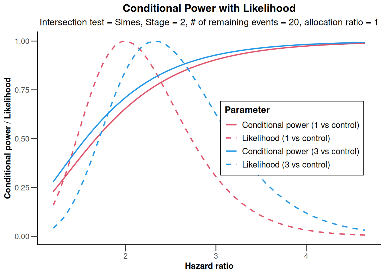

NULL

analysisResultsSurvival |> plot(type = 2)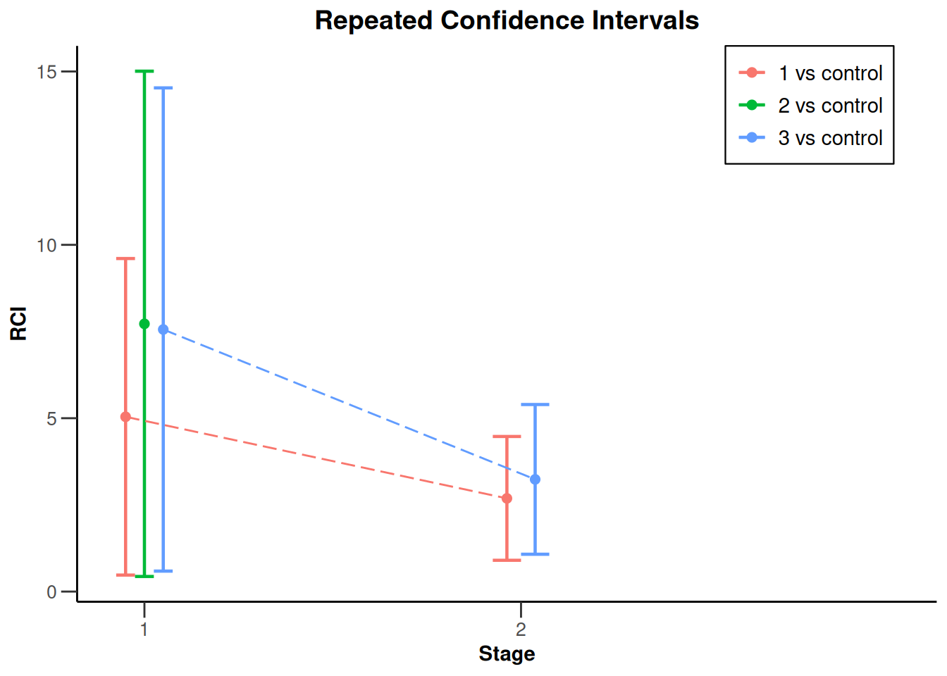

Analysis results enrichment

Analysis results enrichment - means

S1 <- getDataset(
    sampleSize1 = c(14, 22, NA),
    sampleSize2 = c(11, 18, NA),
    mean1       = c(68.3, 107.4, NA),
    mean2       = c(100.1, 140.9, NA),
    stDev1      = c(124.0, 134.7, NA),
    stDev2      = c(116.8, 133.7, NA)
)

S2 <- getDataset(
    sampleSize1 = c(12, NA, NA),
    sampleSize2 = c(18, NA, NA),
    mean1       = c(107.7, NA, NA),
    mean2       = c(125.6, NA, NA),
    stDev1      = c(128.5, NA, NA),
    stDev2      = c(120.1, NA, NA)
)

S3 <- getDataset(
    sampleSize1 = c(17, 24, NA),
    sampleSize2 = c(14, 19, NA),
    mean1       = c(64.3, 101.4, NA),
    mean2       = c(103.1, 170.4, NA),
    stDev1      = c(128.0, 125.3, NA),
    stDev2      = c(111.8, 143.6, NA)
)

F <- getDataset(
    sampleSize1 = c(83, NA, NA),
    sampleSize2 = c(79, NA, NA),
    mean1       = c(77.1, NA, NA),
    mean2       = c(142.4, NA, NA),
    stDev1      = c(163.5, NA, NA),
    stDev2      = c(120.6, NA, NA)
)

dataInput <- getDataset(S1 = S1, S2 = S2, S3 = S3, F = F)

dataInput <- getDataset(S1 = S1, S2 = S2, S12 = S3, R = F)

design <- getDesignInverseNormal(
    kMax = 3, 
    alpha = 0.025, 
    typeOfDesign = "OF",
    informationRates = c(0.2, 0.7, 1)
)

x <- getAnalysisResults(
    design = design,
    dataInput = dataInput,
    directionUpper = FALSE,
    nPlanned = 200
)

x |> plot(populations = c(1, 3))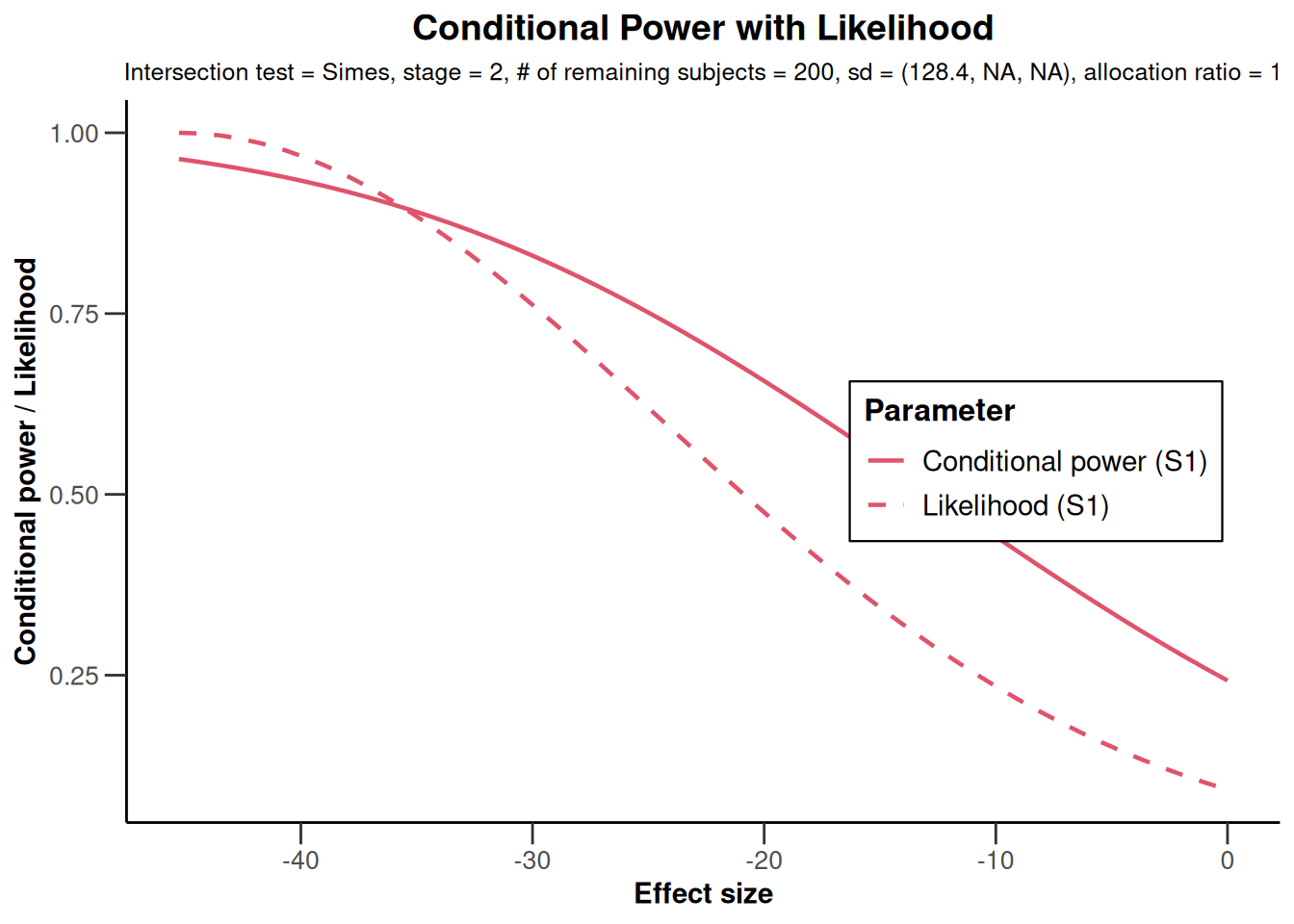

NULL

x |> plot(populations = c(3)) # TODO no output

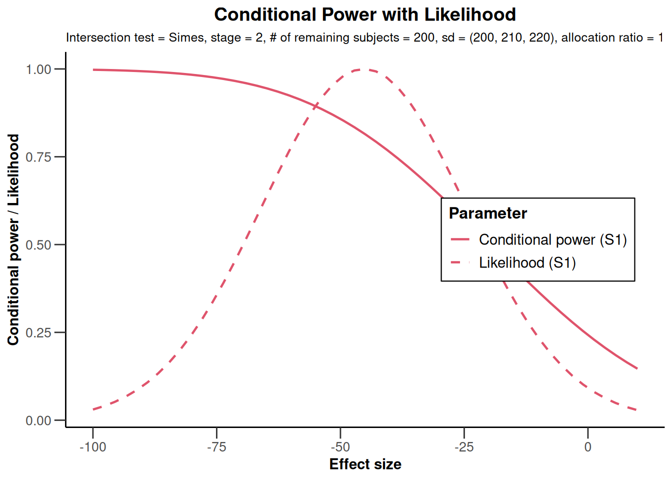
NULL

x |> 
  plot(
    thetaRange = c(-100, 10),
    assumedStDevs = c(200, 210, 220)
)

NULL

x |> plot(type = 2)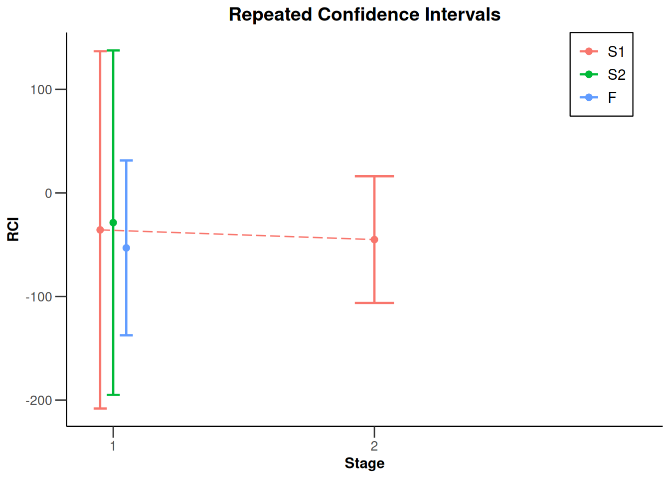

Analysis results enrichment - rates

library(rpact)
S <- getDataset(
    events2 = c(3, 4),
    events1 = c(7, 11),
    n2 = c(30, 31),
    n1 = c(33, 31)
)
R <- getDataset(
    events2 = c(5, 7),
    events1 = c(10, 13),
    n2 = c(32, 30),
    n1 = c(31, 29)
)
dataSetExampleRates <- getDataset(S1 = S, R = R)

x <- getAnalysisResults(
    design = getDesignFisher(),
    dataInput = dataSetExampleRates,
    nPlanned = 30
)
x |> plot()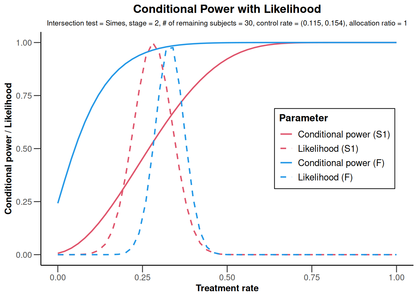

NULL

x |> plot(type = 2)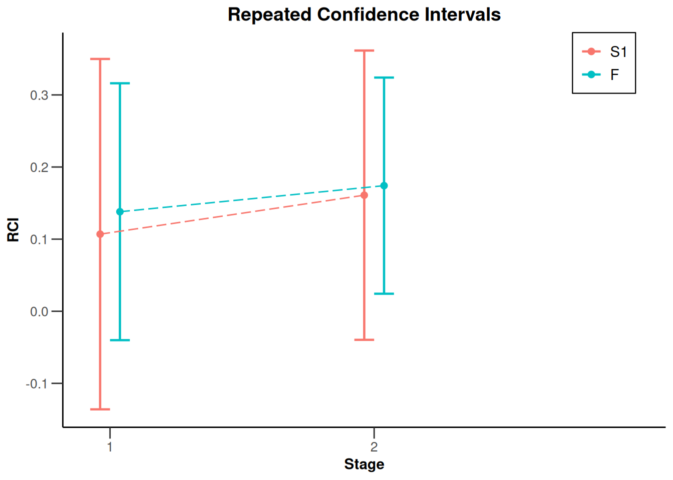

Analysis results enrichment - survival

S <- getDataset(
    events = c(16, 19),
    logRanks = c(1.59, 1.53)
)

F <- getDataset(
    events = c(36, 59),
    logRanks = c(1.98, 1.93)
)
dataSetExampleSurvival <- getDataset(S1 = S, F = F)

x <- getAnalysisResults(
    design = getDesignFisher(),
    dataInput = dataSetExampleSurvival,
    nPlanned = 20
)

Test statistics from full (and sub-populations) need to be stratified log-rank tests

x |> plot()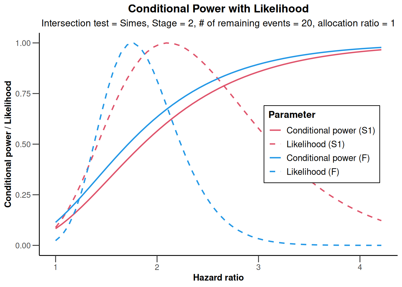

NULL

x |> plot(type = 2)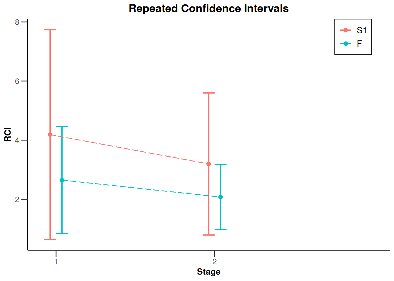

System: rpact 4.3.0.9292, R version 4.5.2 (2025-10-31), platform: x86_64-pc-linux-gnu

To cite R in publications use:

R Core Team (2025). R: A Language and Environment for Statistical Computing. R Foundation for Statistical Computing, Vienna, Austria. https://www.R-project.org/.

To cite package ‘rpact’ in publications use:

Wassmer G, Pahlke F (2025). rpact: Confirmatory Adaptive Clinical Trial Design and Analysis. doi:10.32614/CRAN.package.rpact https://doi.org/10.32614/CRAN.package.rpact, R package version 4.2.0, https://cran.r-project.org/package=rpact.

Reuse

CC BY-SA 4.0