Promizing Zone Design with rpact

Planning, Analysis
We demonstrate how ‘rpact’ enables users to easily define new functions for calculating the number of subjects or events required, based on given conditional power and critical values for specific testing scenarios. This includes the implementation of advanced strategies like the ‘promising zone approach.’
Author
Published

April 16, 2024

Summary

We demonstrate how rpact enables users to easily define new functions for calculating the number of subjects or events required, based on given conditional power and critical values for specific testing scenarios. This includes the implementation of advanced strategies like the ‘promising zone approach.’

A Motivating Example from Hsiao, Liu, and Mehta (Biometrical Journal, 2019)

  • Efficacy endpoint PFS
  • Assumed hazard ratio = 0.67, \(\alpha = 0.025\) and \(\beta = 0.1\) requires 263 events
  • 280 PFS events yields power 91.8 %.

  • If 350 patients are enrolled over 28 months with a median PFS time of 8.5 in the control group, the final analysis is expected to be after an additional follow-up of about 12 months

  • 500 PFS events are needed to have 90% power at HR = 0.75 with more patients and a different expected follow-up

  • “Milestone-based” investment:

    • Two-stage approach with interim after 140 events

    • Enough power for detecting HR = 0.67

    • If conditional power CP for detecting HR = 0.75 falls in a “promizing zone”, an additional investment would be made that allows the trial to remain open until 420 PFS events were obtained

    • Conditional power based on assumed minimum clinical relevant effect HR = 0.75
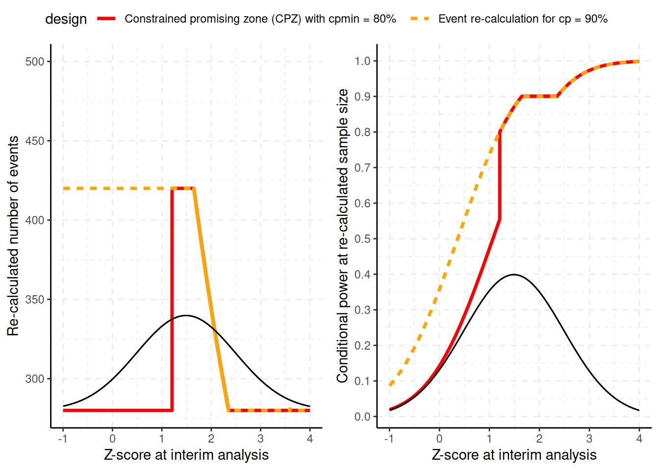
Promizing Zone Design

  • Number of events for the second stage between 140 and 280

  • If conditional power for 280 additional events at HR = 0.75 is smaller than \(cp_{min}\), set number of additional events = 140 (non-promising case)

  • If conditional power for 140 additional events at HR = 0.75 exceeds \(cp_{max}\), set number of additional events = 140, otherwise calculate event number according to \[CP_{HR = 0.75} = cp_{max}\] (promising case)

  • This defined a promizing zone for HR within the sample size may be modified.
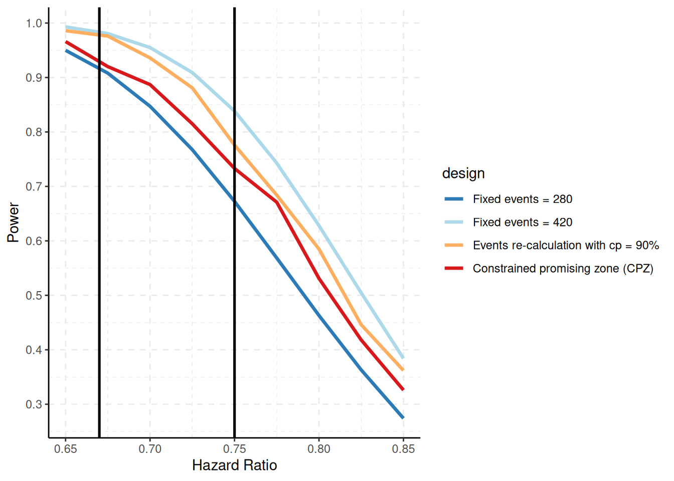
Promizing Zone Design Using rpact

First, define the design

myDesign <- getDesignInverseNormal(kMax = 2, typeOfDesign = "noEarlyEfficacy") 

Define the event number calculation function myEventSizeCalculationFunction()

# Define promizing zone event size function
myEventSizeCalculationFunction <- function(..., stage,
                     plannedEvents,
                     conditionalPower,
                     minNumberOfEventsPerStage,
                     maxNumberOfEventsPerStage,
                     conditionalCriticalValue,
                     estimatedTheta) {
  
  calculateStageEvents <- function(cp) {
      4 * max(0, conditionalCriticalValue + qnorm(cp))^2 / 
      log(max(1 + 1e-12, estimatedTheta))^2
  }
  
  # Calculate events required to reach maximum desired conditional power
  # cp_max (provided as argument conditionalPower)
  stageEventsCPmax <- ceiling(calculateStageEvents(cp = conditionalPower))
  
  # Calculate events required to reach minimum desired conditional power
  # cp_min (**manually set for this example to 0.8**)
  stageEventsCPmin <- ceiling(calculateStageEvents(cp = 0.8))
  
  # Define stageEvents
  stageEvents <- min(max(minNumberOfEventsPerStage[stage], stageEventsCPmax),
    maxNumberOfEventsPerStage[stage])
  
  # Set stageEvents to minimal sample size in case minimum conditional power
  # cannot be reached with available sample size
  if (stageEventsCPmin > maxNumberOfEventsPerStage[stage]) {
    stageEvents <- minNumberOfEventsPerStage[stage]
  
  }
  # return overall events for second stage 
  return(plannedEvents[1] + stageEvents)
}

Run the Simulation

by specifying calcEventsFunction = myEventSizeCalculationFunction and a range of assumed true hazard ratios

hazardRatioSeq <- seq(0.65, 0.85, by = 0.025)
simSurvPromZone <- getSimulationSurvival(design = myDesign,
                      hazardRatio = hazardRatioSeq,
                      directionUpper = FALSE, 
                      plannedEvents = c(140, 280), 
                      median2 = 9,
                      minNumberOfEventsPerStage = c(NA, 140),
                      maxNumberOfEventsPerStage = c(NA, 280),
                      thetaH1 = 0.75,
                      conditionalPower = 0.9,
                      accrualTime = 36, 
                      calcEventsFunction = myEventSizeCalculationFunction,
                      maxNumberOfIterations = maxNumberOfIterations,
                      longTimeSimulationAllowed = TRUE,
                      maxNumberOfSubjects = 500) 

“Usual” Conditional Power Approach

Specify calcEventsFunction = NULL

simSurvCondPower <- getSimulationSurvival(design = myDesign,
                       hazardRatio = hazardRatioSeq, 
                       directionUpper = FALSE, 
                       plannedEvents = c(140, 280), 
                       median2 = 9,
                       minNumberOfEventsPerStage = c(NA, 140),
                       maxNumberOfEventsPerStage = c(NA, 280),
                       thetaH1 = 0.75,
                       conditionalPower = 0.9,
                       accrualTime = 36, 
                       calcEventsFunction = NULL,
                       maxNumberOfIterations = maxNumberOfIterations,
                       longTimeSimulationAllowed = TRUE,
                       maxNumberOfSubjects = 500) 

Comparison of Approaches

aggSimCondPower <- getData(simSurvCondPower)
sumCpower <- summarize(aggSimCondPower, .by = c(iterationNumber, hazardRatio), 
             design = "Event re-calculation for cp = 90%",
             totalSampleSize1 = sum(eventsPerStage), 
             Z1 = testStatistic[1], 
               conditionalPower = conditionalPowerAchieved[2])

aggSimPromZone <- getData(simSurvPromZone)
sumCPZ <- summarize(aggSimPromZone, .by = c(iterationNumber, hazardRatio), 
          design = "Constrained promising zone (CPZ) with cpmin = 80%",
          totalSampleSize1 = sum(eventsPerStage), 
          Z1 = testStatistic[1], 
          conditionalPower = conditionalPowerAchieved[2])

sumBoth <- rbind(sumCpower, sumCPZ) %>%
  filter(Z1 > -1, Z1 < 4)


# Plot it

plot1 <- ggplot(data = sumBoth, aes(Z1, totalSampleSize1, col = design,  group = design)) +
  geom_line(aes(linetype = design), lwd = 1.2) +
  theme_classic() +
  geom_line(aes(Z1, 280 + 150*dnorm(Z1, log(0.75*sqrt(140)/2))), color = "black") +  
  grids(linetype = "dashed") + 
  scale_x_continuous(name = "Z-score at interim analysis") +
  scale_y_continuous(name = "Re-calculated number of events", limits = c(280, 500)) +
  scale_color_manual(values = c("red", "orange"))

plot2 <- ggplot(data = sumBoth, aes(Z1, conditionalPower, col = design, group = design)) +
  geom_line(aes(linetype = design), lwd = 1.2) +
  theme_classic() +
  geom_line(aes(Z1, dnorm(Z1, log(0.75*sqrt(140)/2))), color = "black") +
  grids(linetype = "dashed") + 
  scale_x_continuous(name = "Z-score at interim analysis") +
  scale_y_continuous(
    breaks = seq(0, 1, by = 0.1),
    name = "Conditional power at re-calculated sample size"
  ) +
  scale_color_manual(values = c("red", "orange"))

ggarrange(plot1, plot2, ncol= 2, common.legend = TRUE, legend = "top")

Don’t Increase for, e.g., p = 0.15?

ggplot(data = sumBoth, aes(1 - pnorm(Z1), conditionalPower, col = design, group = design)) +
  geom_line(aes(linetype = design), lwd = 1.2) +
  theme_classic() +
  grids(linetype = "dashed") + 
  scale_x_continuous(name = "p-value at interim analysis") +
  scale_y_continuous(
    breaks = seq(0, 1, by = 0.1),
    name = "Conditional power at re-calculated sample size"
  ) +
  scale_color_manual(values = c("#d7191c", "#fdae61"))

plot(simSurvPromZone, type = 6) 

plot(simSurvCondPower, type = 6)

# Pool datasets from simulations (and fixed designs)
simCondPowerData <- with(as.list(simSurvCondPower),
                      data.frame(
                        design = "Events re-calculation with cp = 90%",
                        hazardRatio = hazardRatio, power = overallReject,
                        expectedNumberOfEvents = expectedNumberOfEvents
                      ))    

simPromZoneData <- with(as.list(simSurvPromZone),
                   data.frame(
                     design = "Constrained promising zone (CPZ)",
                     hazardRatio = hazardRatio, power = overallReject,
                     expectedNumberOfEvents = expectedNumberOfEvents
                   ))

simFixed280 <- data.frame(
                    design = "Fixed events = 280",
                    hazardRatio = hazardRatioSeq,
                    power = getPowerSurvival(alpha = 0.025,
                          directionUpper = FALSE, 
                          maxNumberOfEvents = 280, 
                          median2 = 9,
                          accrualTime = 28, 
                          maxNumberOfSubjects = 500,
                          hazardRatio = hazardRatioSeq
                    )$overallReject,
                    expectedNumberOfEvents = 280
                  )


simFixed420 <- data.frame(
                    design = "Fixed events = 420",
                    hazardRatio = hazardRatioSeq,
                    power = getPowerSurvival(alpha = 0.025,
                           directionUpper = FALSE, 
                           maxNumberOfEvents = 420, 
                           median2 = 9,
                           accrualTime = 28, 
                           maxNumberOfSubjects = 500,
                           hazardRatio = hazardRatioSeq
                    )$overallReject,
                    expectedNumberOfEvents = 420
                  )

simdata <- rbind(simCondPowerData, simPromZoneData, simFixed280, simFixed420)
simdata$design <- factor(simdata$design,
                         levels = c(
                           "Fixed events = 280", 
                           "Fixed events = 420",
                           "Events re-calculation with cp = 90%", 
                           "Constrained promising zone (CPZ)"
                         ))

Difference in Power

# Plot difference in power
ggplot(aes(hazardRatio, power, col = design), data = simdata) +
  theme_classic() +
  grids(linetype = "dashed") + 
  geom_line(lwd = 1.2) +
  scale_x_continuous(name = "Hazard Ratio") +
  scale_y_continuous(breaks = seq(0, 1, by = 0.1), name = "Power") +
  geom_vline(xintercept = c(0.67, 0.75), color = "black", lwd = 0.9) +
  scale_color_manual(values = c("#2c7bb6", "#abd9e9", "#fdae61", "#d7191c"))

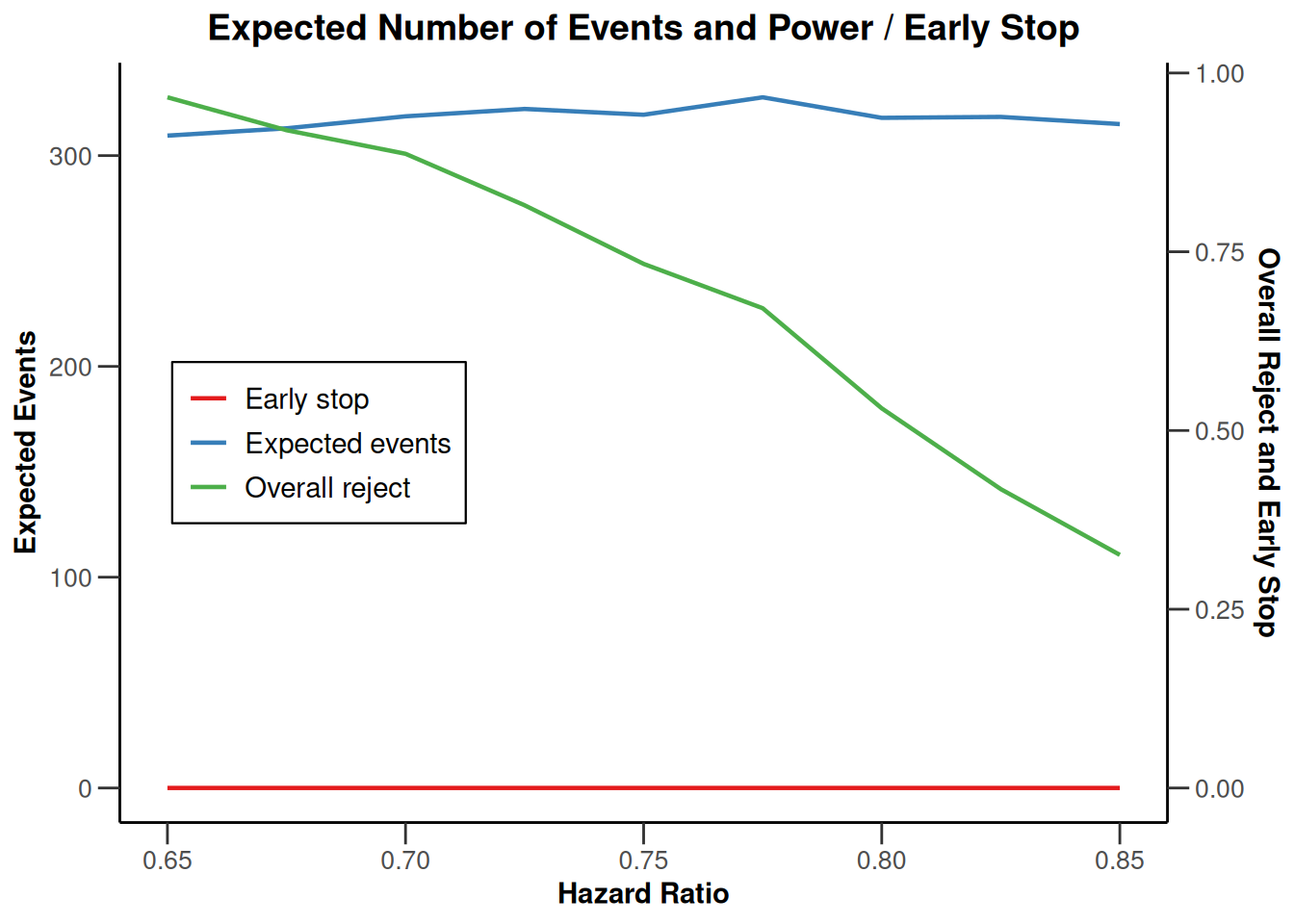
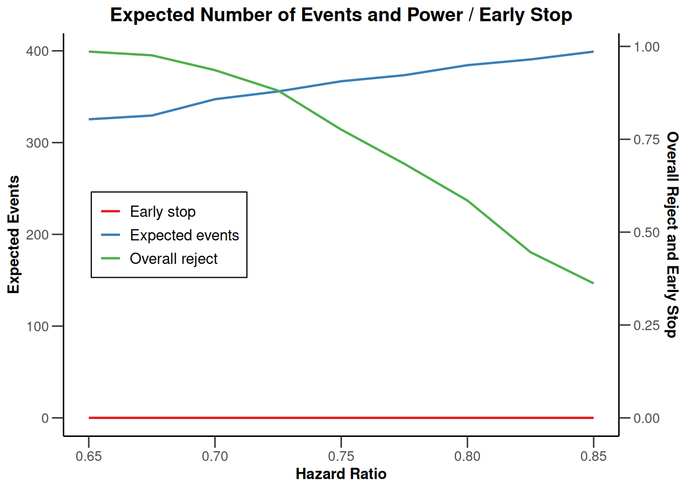
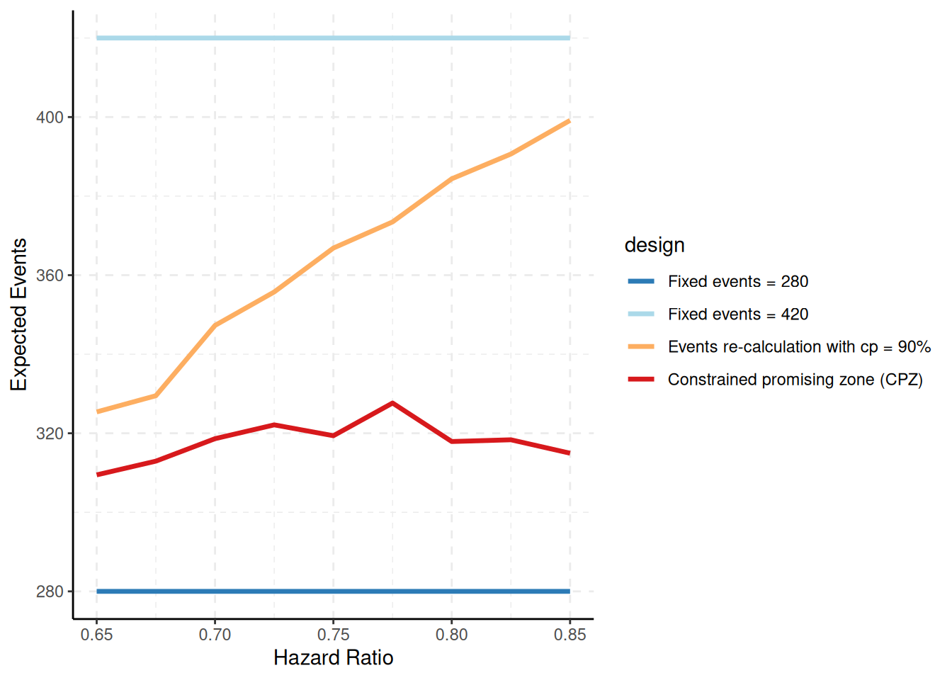
Difference in Expected Sample Size

# Plot difference in expected sample size
ggplot(aes(hazardRatio, expectedNumberOfEvents, col = design), data = simdata) +
  theme_classic() +
  grids(linetype = "dashed") + 
  geom_line(lwd = 1.2) +
  scale_x_continuous(name = "Hazard Ratio") +
  scale_y_continuous(name = "Expected Events") +
  scale_color_manual(values = c("#2c7bb6", "#abd9e9", "#fdae61", "#d7191c"))

Summary

  • Easy implementation in rpact
  • Simulation very fast
  • Consideration of efficacy or futility stops straightforward
  • Trade-off between overall expected sample size and power
  • Usage of combination test (or equivalent) theoretically mandatory
  • Adaptations based on test statistic only

References

Wassmer, G and Brannath, W. Group Sequential and Confirmatory Adaptive Designs in Clinical Trials (2016), ISBN 978-3319325606 https://doi.org/10.1007/978-3-319-32562-0


System rpact 4.0.0, R version 4.3.3 (2024-02-29 ucrt), platform x86_64-w64-mingw32

To cite R in publications use:

R Core Team (2024). R: A Language and Environment for Statistical Computing. R Foundation for Statistical Computing, Vienna, Austria. https://www.R-project.org/. To cite package ‘rpact’ in publications use:

Wassmer G, Pahlke F (2024). rpact: Confirmatory Adaptive Clinical Trial Design and Analysis. R package version 4.0.0, https://www.rpact.com, https://github.com/rpact-com/rpact, https://rpact-com.github.io/rpact/, https://www.rpact.org.