Designing Group Sequential Trials with Two Groups and a Survival Endpoint with rpact

Planning

Survival

This document provides examples for designing trials with survival endpoints using rpact.

Author

Marcel Wolbers Gernot Wassmer Friedrich Pahlke

Published

October 28, 2024

Introduction

The examples in this document are not intended to replace the official rpact documentation and help pages but rather to supplement them. They also only cover a selection of all rpact features.

General convention: In rpact, arguments containing the index “2” always refer to the control group, “1” refer to the intervention group, and treatment effects compare treatment versus control.

First, load the rpact package

library(rpact)
packageVersion("rpact")

[1] '4.1.1'

Overview of relevant rpact functions

The sample size calculation for a group sequential trial with a survival endpoints is performed in two steps:

Define the (abstract) group sequential design using the function getDesignGroupSequential(). For details regarding this step, see the R markdown file Defining group sequential boundaries with rpact. This step can be omitted if the trial has no interim analyses.
Calculate sample size for the survival endpoint by feeding the abstract design into the function getSampleSizeSurvival(). This step is described in detail below.

Other relevant rpact functions for survival are:

getPowerSurvival(): This function is the analogue to getSampleSizeSurvival() for the calculation of power rather than the sample size.
getEventProbabilities(): Calculates the probability of an event depending on the time and type of accrual, follow-up time, and survival distribution. This is useful for aligning interim analyses for different time-to-event endpoints.
getSimulationSurvival(): This function simulates group sequential trials. For example, it allows to assess the power of trials with delayed treatment effects or to assess the data-dependent variability of the timing of interim analyses even if the protocol assumptions are perfectly fulfilled. It also allows to simulate hypothetical datasets for trials stopped early.

This document describes all functions mentioned above except for trial simulation (getSimulationSurvival()) which is described in the document Simulation-based design of group sequential trials with a survival endpoint with rpact.

However, before describing the functions themselves, the document describes how survival functions, drop-out, and accrual can be specified in rpact which is required for all of these functions.

Specifying survival distributions in rpact

rpact allows to specify survival distributions with exponential, piecewise exponential, and Weibull distributions. Exponential and piecewise exponential distributions are described below.

Weibull distributions are specified in the same way as exponential distributions except that an additional scale parameter kappa needs to be provided which is 1 for the exponential distribution. Note that the parameters shape and scale in the standard R functions for the Weibull distribution in the stats-library (such as dweibull) are equivalent to kappa and 1/lambda, respectively, in rpact.

Exponential survival distributions

Event probability at a specific time point known

The time point is given by argument eventTime.
The probability of an event (i.e., 1 minus survival function) in the control group is given by argument pi2.
The probability of an event in the intervention arm can either be provided explicitly through argument pi1 or, alternatively, implicitly by specifying the target hazard ratio hazardRatio.

Example: If the intervention is expected to improve survival at 24 months from 70% to 80%, this would be expressed through arguments eventTime = 24, pi2 = 0.3, pi1 = 0.2.

Exponential parameter $\lambda$ known

The constant hazard function in the control arm can be provided as argument lambda2.
The hazard in the intervention arm can either be provided explicitly through the argument lambda1 or, alternatively, implicitly by specifying the target hazard ratio hazardRatio.

Median survival known

Medians cannot be specified directly. However, one can exploit that the hazard rate $\lambda$ of the exponential distribution is equal to $\lambda = \log(2)/\text{median}$.

Example: If the intervention is expected to improve the median survival from 60 to 75 months, this would be expressed through the arguments lambda2 = log(2)/60, lambda1 = log(2)/75. Alternatively, it could be specified via lambda2 = log(2)/60, hazardRatio = 0.8 (as the hazard ratio is 60/75 = 0.8).

Weibull

Weibull distributions are specified in the same way as exponential distributions except that an additional scale parameter kappa needs to be provided which is 1 for the exponential distribution.

Piecewise exponential survival

Piecewise constant hazard rate $\lambda$ in each interval known

Example: If the survival function in the control arm is assumed to be 0.03 (events/time-unit of follow-up) for the first 6 months, 0.06 for months 6-12, and 0.02 from month 12 onwards, this can be specified using the argument piecewiseSurvivalTime as follows:

piecewiseSurvivalTime = list(
    "0 - <6" = 0.03,
    "6 - <12" = 0.06,
    ">= 12" = 0.02)

Alternatively, the same distribution can be specified by giving the start times of each interval as argument piecewiseSurvivalTime and the actual hazard rate in that interval as argument lambda2. I.e., the relevant arguments for this example would be:

piecewiseSurvivalTime = c(0,6,12), lambda2 = c(0.03,0.06,0.02)

For the intervention arm, one could either explicitly specify the hazard rate in the same time intervals through the argument lambda1 or, more conveniently, specify the survival function in the intervention arm indirectly via the target hazard ratio (argument hazardRatio).

Note: The sample size calculation functions discussed in this document assume that the proportional hazards assumption holds, i.e., that lambda1 and lambda2 are proportional if both are provided. Otherwise, the function call to getSampleSizeSurvival() gives an error. For situations with non-proportional hazards, please see the separate document which discusses the simulation tool using the function getSimulationSurvival().

Survival function at different time points known

Piecewise exponential distributions are useful to approximate survival functions. In principle, it is possible to approximate any distribution function well with a piecewise exponential distribution if suitably narrow intervals are chosen.

Assume that the survival function is $S(t_1)$ at time $t_1$ and $S(t_2)$ at time $t_2$ with $t_2>t_1$ and that the hazard rate in the interval $[t_1,t_2]$ is constant. Then, the hazard rate in the interval can be derived as $(\log(S(t_1))-\log(S(t_2)))/(t_2-t_1)$.

Example: Assume that it is known that the survival function is 1, 0.9, 0.7, and 0.5 at months 0, 12, 24, 48 in the control arm. Then, an interpolating piecewise exponential distribution can be derived as follows:

t <- c(0, 12, 24, 48) # time points at which survival function is known
# (must include 0)
S <- c(1, 0.9, 0.7, 0.5) # Survival function at timepoints t
# derive hazard in each intervals per the formula above
lambda <- -diff(log(S)) / diff(t)
# Define parameters for piecewise exponential distribution in the control arm
# interpolating the targeted survival values
# (code for lambda1 below assumes that the hazard afer month 48 is
#  identical to the hazard in interval [24,48])
piecewiseSurvivalTime <- t
lambda2 <- c(lambda, tail(lambda, n = 1))
lambda2 # print hazard rates

[1] 0.008780043 0.020942869 0.014019677 0.014019677

Appendix: Random numbers, cumulative distribution, and quantiles for the piecewise exponential distribution

rpact also provides general functionality for the piecewise exponential distribution, see ?getPiecewiseExponentialDistribution for details. Below is some example code which shows that the derivation of the piecewise exponential distribution in the previous example is correct.

# plot the piecewise exponential survival distribution from the example above
tp <- seq(0, 72, by = 0.01)
plot(tp,
    1 - getPiecewiseExponentialDistribution(
        time = tp,
        piecewiseSurvivalTime = piecewiseSurvivalTime,
        piecewiseLambda = lambda2
    ),
    type = "l", 
    xlab = "Time (months)", 
    ylab = "Survival function S(t)",
    lwd = 2, 
    ylim = c(0, 1), 
    axes = FALSE,
    main = "Piecewise exponential distribution for the example"
)
axis(1, at = seq(0, 72, by = 12))
axis(2, at = seq(0, 1, by = 0.1))
abline(v = seq(0, 72, by = 12), h = seq(0, 1, by = 0.1), col = gray(0.9))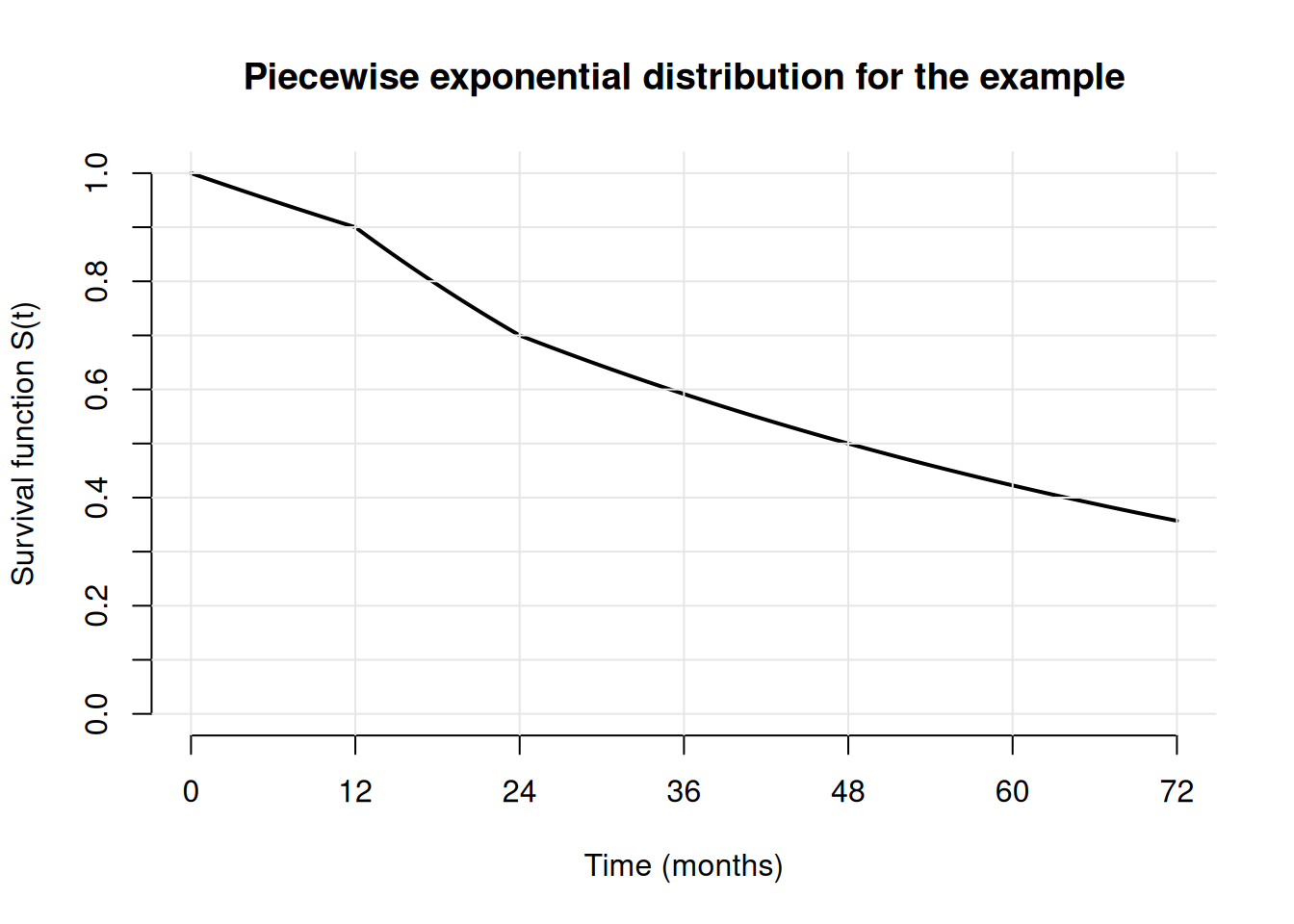

# Calculate median survival for the example (which should give 48 months here)
getPiecewiseExponentialQuantile(0.5,
    piecewiseSurvivalTime = piecewiseSurvivalTime,
    piecewiseLambda = lambda2
)

[1] 48

Specifying dropout in rpact

rpact models dropout with an independent exponentially distributed variable. Dropout is specified by giving the probability of dropout at a specific time point. For example, an annual (12-monthly) dropout probability of 5% in both treatment arms can be specified through the following arguments:

dropoutRate1 = 0.05, dropoutRate2 = 0.05, dropoutTime = 12

Specifying accrual in rpact

rpact allows to specify arbitrarily complex recruitment scenarios. Some examples are provided below.

Absolute accrual intensity and accrual duration known

Example 1: A constant accrual intensity of 24 subjects/months over 30 months (i.e., a maximum sample size of 24*30 = 720 subjects) can be specified through the arguments below:

accrualTime = c(0, 30), accrualIntensity = 24

Example 2: A flexible accrual intensity of 20 subjects/months in the first 6 months, 25 subjects/months for months 6-12, and 30 subjects per month for months 12-24 can be specified through either of the two equivalent options below:

Option 1: List-based definition:

accrualTime = list(
    "0 - <6" = 20,
    "6 - <12" = 25,
    "12- <24" = 30)

Option 2: Vector-based definition (note that the length of the accrualTime vector is 1 larger than the length of the accrualIntensity as the end time of the accrual period is also included):

accrualTime = c(0, 6, 12, 24), accrualIntensity = c(20, 25, 30)

Absolute accrual intensity known, accrual duration unknown

Example 1: A constant accrual intensity of 24 subjects/months with unspecified end of recruitment is specified through the arguments below:

accrualTime = 0, accrualIntensity = 24 
# Note: accrualTime is the start of accrual which must be explicitly set to 0

Example 2: A flexible accrual intensity of 20 subjects/months in the first 6 months, 25 subjects/months from month 6-12, and 30 subjects thereafter can be specified through either of the two equivalent options below:

Option 1: List-based definition:

accrualTime = list(
    "0 - <6" = 20,
    "6 - <12" = 25,
    ">= 12" = 30)

Option 2: Vector-based definition (note that the length of the accrualTime vector is equal to the length of the accrualIntensity vector as only the start time of the last accrual intensity is provided):

accrualTime = c(0, 6, 12), accrualIntensity = c(20, 25, 30)

Sample size calculation for superiority trials without interim analyses

Given the specification of the survival distributions, drop-out and accrual as described above, sample size calculations can be readily performed in rpact using the function getSampleSizeSurvival(). Importantly, in survival trials, the number of events (and not the sample size) determines the power of the trial. Hence, the choice of the sample size to reach this target number of events is based on study-specific trade-offs between the costs per recruited patient, study duration, and desired minimal follow-up duration.

In practice, a range of sample sizes need to be explored manually or via suitable graphs to find an optimal trade off. Given a plausible absolute accrual intensity (usually provided by operations), a simple approach in rpact is to use one or both of the two options below:

Perform the calculation by trying multiple maximum sample sizes (argument maxNumberOfSubjects).
It often makes sense to require a minimal follow-up time (argument followUpTime) for all patients in the trial at the time of the analysis. In this case, rpact automatically determines the maximum sample size.

Example - exponential survival, flexible accrual intensity, no interim analyses

Exponential PFS with a median PFS of 60 months in control (lambda2 = log(2)/60) and a target hazard ratio of 0.74 (hazardRatio = 0.74).
Log-rank test at the two-sided 5%-significance level (sided = 2, alpha = 0.05), power 80% (beta = 0.2).
Annual drop-out of 2.5% in both arms (dropoutRate1 = 0.025, dropoutRate2 = 0.025, dropoutTime = 12).
Recruitment is 42 patients/month from month 6 onwards after linear ramp up. (accrualTime = c(0,1,2,3,4,5,6), accrualIntensity = c(6,12,18,24,30,36,42))
Randomization ratio 1:1 (allocationRatioPlanned = 1). This is the default and is thus not explicitly set in the function call below.
Two sample size choices will be initially explored:
- A fixed total sample size of 1200 (maxNumberOfSubjects = 1200).
- Alternatively, the total sample size will be implicitly determined by specifying that every subject must have a minimal follow-up duration of at 12 months at the time of the analysis (followUpTime = 12).

Based on this, the required number of events and timing of interim analyses for the fixed total sample size of 1200 can be determined as follows:

sampleSize1 <- getSampleSizeSurvival(
    sided = 2, 
    alpha = 0.05, 
    beta = 0.2,
    lambda2 = log(2) / 60, 
    hazardRatio = 0.74,
    dropoutRate1 = 0.025, 
    dropoutRate2 = 0.025, 
    dropoutTime = 12,
    accrualTime = c(0, 1, 2, 3, 4, 5, 6),
    accrualIntensity = c(6, 12, 18, 24, 30, 36, 42),
    maxNumberOfSubjects = 1200
)
sampleSize1

Design plan parameters and output for survival data

Design parameters

Critical values: 1.960
Two-sided power: FALSE
Significance level: 0.0500
Type II error rate: 0.2000
Test: two-sided

User defined parameters

lambda(2): 0.0116
Hazard ratio: 0.740
Maximum number of subjects: 1200
Accrual time: 1.00, 2.00, 3.00, 4.00, 5.00, 6.00, 31.57
Accrual intensity: 6.0, 12.0, 18.0, 24.0, 30.0, 36.0, 42.0
Drop-out rate (1): 0.025
Drop-out rate (2): 0.025

Default parameters

Theta H0: 1
Type of computation: Schoenfeld
Planned allocation ratio: 1
kappa: 1
Piecewise survival times: 0.00
Drop-out time: 12.00

Sample size and output

Direction upper: FALSE
median(1): 81.1
median(2): 60.0
lambda(1): 0.00855
Number of events: 346.3
Total accrual time: 31.57
Follow up time: 21.54
Number of events fixed: 346.3
Number of subjects fixed: 1200
Number of subjects fixed (1): 600
Number of subjects fixed (2): 600
Analysis time: 53.11
Study duration: 53.11
Lower critical values (treatment effect scale): 0.810
Upper critical values (treatment effect scale): 1.234

Legend

(i): values of treatment arm i

Thus, the required number of events is 347 and the MDD corresponds to observed HR of 0.81 or 1.23, respectively. The 1200 subjects will be recruited over 31.57 months and the total study duration is 53.11 months. The user could now vary maxNumberSubject to further optimize the trade-off between sample size and study duration.

Alternatively, specifying a minimum follow-up duration of 12 months leads to the following result:

sampleSize2 <- getSampleSizeSurvival(
    sided = 2, 
    alpha = 0.05, 
    beta = 0.2,
    lambda2 = log(2) / 60, 
    hazardRatio = 0.74,
    dropoutRate1 = 0.025, 
    dropoutRate2 = 0.025, 
    dropoutTime = 12,
    accrualTime = c(0, 1, 2, 3, 4, 5, 6),
    accrualIntensity = c(6, 12, 18, 24, 30, 36, 42),
    followUpTime = 12
)
sampleSize2

Design plan parameters and output for survival data

Design parameters

Critical values: 1.960
Two-sided power: FALSE
Significance level: 0.0500
Type II error rate: 0.2000
Test: two-sided

User defined parameters

lambda(2): 0.0116
Hazard ratio: 0.740
Accrual intensity: 6.0, 12.0, 18.0, 24.0, 30.0, 36.0, 42.0
Follow up time: 12.00
Drop-out rate (1): 0.025
Drop-out rate (2): 0.025

Default parameters

Theta H0: 1
Type of computation: Schoenfeld
Planned allocation ratio: 1
kappa: 1
Piecewise survival times: 0.00
Drop-out time: 12.00

Sample size and output

Direction upper: FALSE
median(1): 81.1
median(2): 60.0
lambda(1): 0.00855
Maximum number of subjects: 1433.7
Number of events: 346.3
Accrual time: 1.00, 2.00, 3.00, 4.00, 5.00, 6.00, 37.13
Total accrual time: 37.13
Number of events fixed: 346.3
Number of subjects fixed: 1433.7
Number of subjects fixed (1): 716.8
Number of subjects fixed (2): 716.8
Analysis time: 49.13
Study duration: 49.13
Lower critical values (treatment effect scale): 0.810
Upper critical values (treatment effect scale): 1.234

Legend

(i): values of treatment arm i

This specification leads to a higher sample size of 1434 subjects which will be recruited over 37.13 months and the total study duration is 49.13 months.

With the generic summary() function the two calculations are summarized as follows:

sampleSize1 |> summary()

Sample size calculation for a survival endpoint

Fixed sample analysis, two-sided significance level 5%, power 80%. The results were calculated for a two-sample logrank test, H0: hazard ratio = 1, H1: hazard ratio = 0.74, control lambda(2) = 0.012, number of subjects = 1200, accrual time = c(1, 2, 3, 4, 5, 6, 31.571), accrual intensity = c(6, 12, 18, 24, 30, 36, 42), dropout rate(1) = 0.025, dropout rate(2) = 0.025, dropout time = 12.

Stage	Fixed
Stage level (two-sided)	0.0500
Efficacy boundary (z-value scale)	1.960
Lower efficacy boundary (t)	0.810
Upper efficacy boundary (t)	1.234
Number of subjects	1200.0
Number of events	346.3
Analysis time	53.11
Expected study duration under H1	53.11

Legend:

(t): treatment effect scale

sampleSize2 |> summary()

Sample size calculation for a survival endpoint

Fixed sample analysis, two-sided significance level 5%, power 80%. The results were calculated for a two-sample logrank test, H0: hazard ratio = 1, H1: hazard ratio = 0.74, control lambda(2) = 0.012, accrual time = c(1, 2, 3, 4, 5, 6, 37.135), accrual intensity = c(6, 12, 18, 24, 30, 36, 42), follow-up time = 12, dropout rate(1) = 0.025, dropout rate(2) = 0.025, dropout time = 12.

Stage	Fixed
Stage level (two-sided)	0.0500
Efficacy boundary (z-value scale)	1.960
Lower efficacy boundary (t)	0.810
Upper efficacy boundary (t)	1.234
Number of subjects	1433.7
Number of events	346.3
Analysis time	49.13
Expected study duration under H1	49.13

Legend:

(t): treatment effect scale

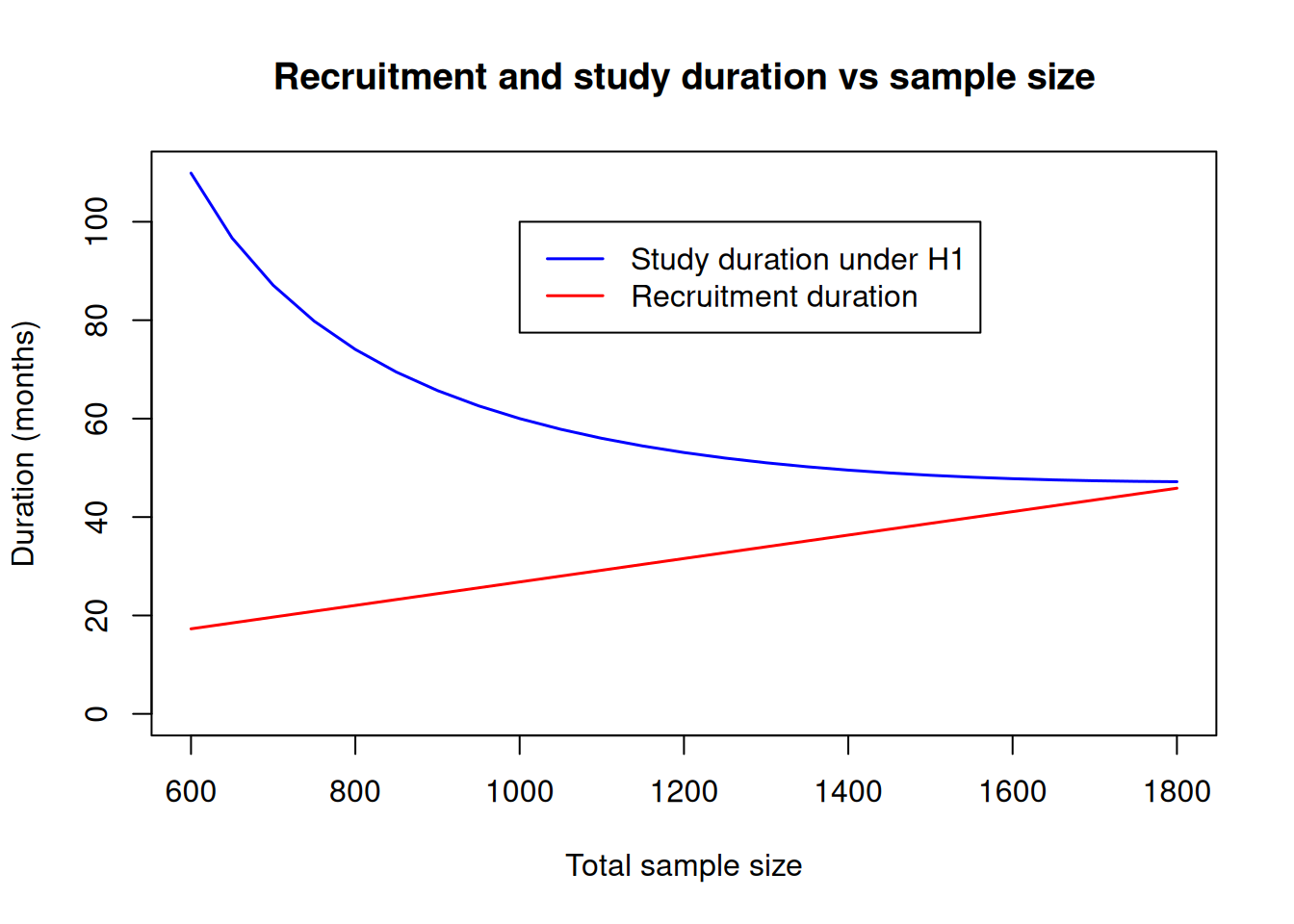
To further explore the possible trade-offs, one could visualize recruitment and study durations for a range of sample sizes as illustrated in the code below:

# set up data frame which contains sample sizes and corresponding durations
sampleSizeDuration <- data.frame(
    maxNumberSubjects = seq(600, 1800, by = 50),
    accrualTime = NA,
    studyDuration = NA
)

# calculate recruitment and study duration for each sample size
for (i in 1:nrow(sampleSizeDuration)) {
    sampleSizeResult <- getSampleSizeSurvival(
        sided = 2, 
        alpha = 0.05, 
        beta = 0.2,
        lambda2 = log(2) / 60, 
        hazardRatio = 0.74,
        dropoutRate1 = 0.025, 
        dropoutRate2 = 0.025, 
        dropoutTime = 12,
        accrualTime = c(0, 1, 2, 3, 4, 5, 6),
        accrualIntensity = c(6, 12, 18, 24, 30, 36, 42),
        maxNumberOfSubjects = sampleSizeDuration$maxNumberSubjects[i]
    )
    sampleSizeDuration$accrualTime[i] <- sampleSizeResult$totalAccrualTime
    sampleSizeDuration$studyDuration[i] <- sampleSizeResult$maxStudyDuration
}

# plot result
plot(sampleSizeDuration$maxNumberSubjects,
    sampleSizeDuration$studyDuration,
    type = "l",
    xlab = "Total sample size",
    ylab = "Duration (months)",
    main = "Recruitment and study duration vs sample size",
    ylim = c(0, max(sampleSizeDuration$studyDuration)),
    col = "blue", lwd = 1.5
)
lines(sampleSizeDuration$maxNumberSubjects,
    sampleSizeDuration$accrualTime,
    col = "red", lwd = 1.5
)
legend(
    x = 1000, y = 100,
    legend = c(
        "Study duration under H1",
        "Recruitment duration"
    ),
    col = c("blue", "red"), lty = 1, lwd = 1.5
)

Sample size calculation for non-inferiority trials without interim analyses

Sample size calculation proceeds in the same fashion as for superiority trials except that the role of the null and the alternative hypothesis are reversed. I.e., in this case, the non-inferiority margin $\Delta$ corresponds to the treatment effect under the null hypothesis (thetaH0). Testing for non-inferiority trials is always one-sided.

In the example code below, we assume that the non-inferiority margin corresponds to a 20% increase of the hazard function and that “in reality”, i.e., under the alternative hypothesis, the survival functions in the two groups are equal. In this case, the “null hypothesis” is thetaH0 = 1.2 versus the “alternative” hazardRatio = 1. For illustration, all other assumptions were chosen as per the sample size calculations for superiority trials above.

sampleSizeNonInf <- getSampleSizeSurvival(
    sided = 1, 
    alpha = 0.025, 
    beta = 0.2,
    lambda2 = log(2) / 60,
    thetaH0 = 1.2, 
    hazardRatio = 1,
    dropoutRate1 = 0.025, 
    dropoutRate2 = 0.025, 
    dropoutTime = 12,
    accrualTime = c(0, 1, 2, 3, 4, 5, 6),
    accrualIntensity = c(6, 12, 18, 24, 30, 36, 42),
    followUpTime = 12
)

sampleSizeNonInf

Design plan parameters and output for survival data

Design parameters

Critical values: 1.960
Significance level: 0.0250
Type II error rate: 0.2000
Test: one-sided

User defined parameters

Theta H0: 1.2
lambda(2): 0.0116
Hazard ratio: 1.000
Accrual intensity: 6.0, 12.0, 18.0, 24.0, 30.0, 36.0, 42.0
Follow up time: 12.00
Drop-out rate (1): 0.025
Drop-out rate (2): 0.025

Default parameters

Type of computation: Schoenfeld
Planned allocation ratio: 1
kappa: 1
Piecewise survival times: 0.00
Drop-out time: 12.00

Sample size and output

Direction upper: FALSE
median(1): 60.0
median(2): 60.0
lambda(1): 0.0116
Maximum number of subjects: 2609.2
Number of events: 944.5
Accrual time: 1.00, 2.00, 3.00, 4.00, 5.00, 6.00, 65.12
Total accrual time: 65.12
Number of events fixed: 944.5
Number of subjects fixed: 2609.2
Number of subjects fixed (1): 1304.6
Number of subjects fixed (2): 1304.6
Analysis time: 77.12
Study duration: 77.12
Critical values (treatment effect scale): 1.056

Legend

(i): values of treatment arm i

In this example, the required number of events is 945. The specification above leads to a sample size of 2610 subjects recruited over 65.12 months and an expected total study duration of 77.12 months.

Sample size calculation for trials with interim analyses

Calculations can be performed as for trials without interim analyses except that the group sequential design needs to be specified using getDesignGroupSequential before calling getSampleSizeSurvival. For details regarding the specification of the group sequential design, see the R Markdown file Defining group sequential boundaries with rpact.

In general, rpact supports both one-sided and two-sided group sequential designs. However, if futility boundaries are specified, only one-sided tests are permitted. For simplicity, it is often preferred to use one-sided tests for group sequential designs (typically with $\alpha = 0.025$).

One additional consideration for phase III trials with efficacy interim analyses is that they should only be performed at time-points when the data is sufficiently mature to allow for a potential filing. For example, it is often sensible to perform efficacy interim analyses only after all subjects have been recruited. This aspect can be further explored by looking at simulated data for (hypothetical) trials that would have stopped at the interim analysis. This can easily be implemented using the simulation tool in rpact and we refer to the R Markdown document Simulation-based design of group sequential trials with a survival endpoint with rpact for further details.

Example - piece-wise exponential survival, constant accrual intensity, group sequential design

1:1 randomized.
80% power at the one-sided 2.5% significance level.
Efficacy interim analyses at 50% and 75% of total information using an O’Brien & Fleming type $\alpha$-spending function, no futility interim analyses.
Target HR for primary endpoint (PFS) is 0.75.
PFS in the control arm follows a piece-wise exponential distribution, with the hazard rate h(t) estimated using historical controls as follows:
- h(t) = 0.025 for t between 0 and 6 months,
- h(t) = 0.04 for t between 6 and 9 months,
- h(t) = 0.015 for t between 9 and 15 months,
- h(t) = 0.01 for t between 15 and 21 months,
- h(t) = 0.007 for t beyond 21 months.
An annual dropout probability of 5%.
Recruitment of 42 patients/month up to a maximum of 1000 subjects.

Sample size calculation

The group sequential design (including Type I and II error) can be specified as follows:

design <- getDesignGroupSequential(
    sided = 1, 
    alpha = 0.025, 
    beta = 0.2,
    informationRates = c(0.5, 0.75, 1),
    typeOfDesign = "asOF"
)

The piecewise exponential survival is defined as described above:

piecewiseSurvivalTime <- list(
    "0 - <6" = 0.025,
    "6 - <9" = 0.04,
    "9 - <15" = 0.015,
    "15 - <21" = 0.01,
    ">= 21" = 0.007
)

Now, the sample size calculation can be performed:

sampleSizeResult <- getSampleSizeSurvival(
    design = design,
    piecewiseSurvivalTime = piecewiseSurvivalTime, 
    hazardRatio = 0.75,
    dropoutRate1 = 0.05, 
    dropoutRate2 = 0.05, 
    dropoutTime = 12,
    accrualTime = 0, 
    accrualIntensity = 42, 
    maxNumberOfSubjects = 1000
)

The sample size result can be summarized by displaying the default rpact output:

sampleSizeResult

Design plan parameters and output for survival data

Design parameters

Information rates: 0.500, 0.750, 1.000
Critical values: 2.963, 2.359, 2.014
Futility bounds (non-binding): -Inf, -Inf
Cumulative alpha spending: 0.001525, 0.009649, 0.025000
Local one-sided significance levels: 0.001525, 0.009162, 0.022000
Significance level: 0.0250
Type II error rate: 0.2000
Test: one-sided

User defined parameters

Piecewise survival lambda (2): 0.025, 0.040, 0.015, 0.010, 0.007
Hazard ratio: 0.750
Maximum number of subjects: 1000
Accrual time: 23.81
Accrual intensity: 42.0
Piecewise survival times: 0.00, 6.00, 9.00, 15.00, 21.00
Drop-out rate (1): 0.050
Drop-out rate (2): 0.050

Default parameters

Theta H0: 1
Type of computation: Schoenfeld
Planned allocation ratio: 1
kappa: 1
Drop-out time: 12.00

Sample size and output

Direction upper: FALSE
Piecewise survival lambda (1): 0.01875, 0.03000, 0.01125, 0.00750, 0.00525
Maximum number of subjects (1): 500
Maximum number of subjects (2): 500
Number of subjects [1]: 973.2
Number of subjects [2]: 1000
Number of subjects [3]: 1000
Maximum number of events: 386.8
Follow up time: 36.19
Reject per stage [1]: 0.1680
Reject per stage [2]: 0.3720
Reject per stage [3]: 0.2600
Early stop: 0.5400
Analysis time [1]: 23.17
Analysis time [2]: 33.28
Analysis time [3]: 60.00
Expected study duration: 43.87
Maximal study duration: 60.00
Cumulative number of events [1]: 193.4
Cumulative number of events [2]: 290.1
Cumulative number of events [3]: 386.8
Expected number of events under H0: 385.7
Expected number of events under H0/H1: 371.7
Expected number of events under H1: 318.3
Expected number of subjects under H1: 995.5
Critical values (treatment effect scale) [1]: 0.653
Critical values (treatment effect scale) [2]: 0.758
Critical values (treatment effect scale) [3]: 0.815

Legend

(i): values of treatment arm i
[k]: values at stage k

In addition, the generic summary() function summarizes the results per stage in a different format and also adds results which are stored in the underlying group sequential design such as exit probabilities:

# Summarize design
sampleSizeResult |> summary()

Sample size calculation for a survival endpoint

Sequential analysis with a maximum of 3 looks (group sequential design), one-sided overall significance level 2.5%, power 80%. The results were calculated for a two-sample logrank test, H0: hazard ratio = 1, H1: hazard ratio = 0.75, piecewise survival distribution, piecewise survival time = c(0, 6, 9, 15, 21), control lambda(2) = c(0.025, 0.04, 0.015, 0.01, 0.007), maximum number of subjects = 1000, accrual time = 23.81, accrual intensity = 42, dropout rate(1) = 0.05, dropout rate(2) = 0.05, dropout time = 12.

Stage	1	2	3
Planned information rate	50%	75%	100%
Cumulative alpha spent	0.0015	0.0096	0.0250
Stage levels (one-sided)	0.0015	0.0092	0.0220
Efficacy boundary (z-value scale)	2.963	2.359	2.014
Efficacy boundary (t)	0.653	0.758	0.815
Cumulative power	0.1680	0.5400	0.8000
Number of subjects	973.2	1000.0	1000.0
Expected number of subjects under H1			995.5
Cumulative number of events	193.4	290.1	386.8
Expected number of events under H1			318.3
Analysis time	23.17	33.28	60.00
Expected study duration under H1			43.87
Exit probability for efficacy (under H0)	0.0015	0.0081
Exit probability for efficacy (under H1)	0.1680	0.3720

Legend:

(t): treatment effect scale

Sample size plots

rpact provides a large number of plots, see the R Markdown document How to create admirable plots with rpact for examples of all plots. Below, we just show two selected plots.

# Boundary on treatment effect scale
sampleSizeResult |> plot(type = 2, showSource = TRUE)

Source data of the plot (type 2):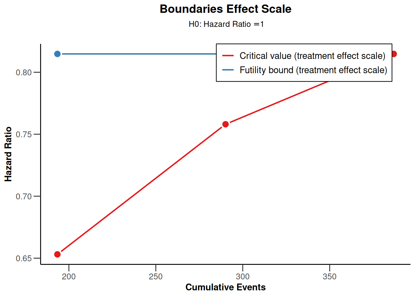

# Survival function and piecewise constant hazard
sampleSizeResult |> plot(type = 14)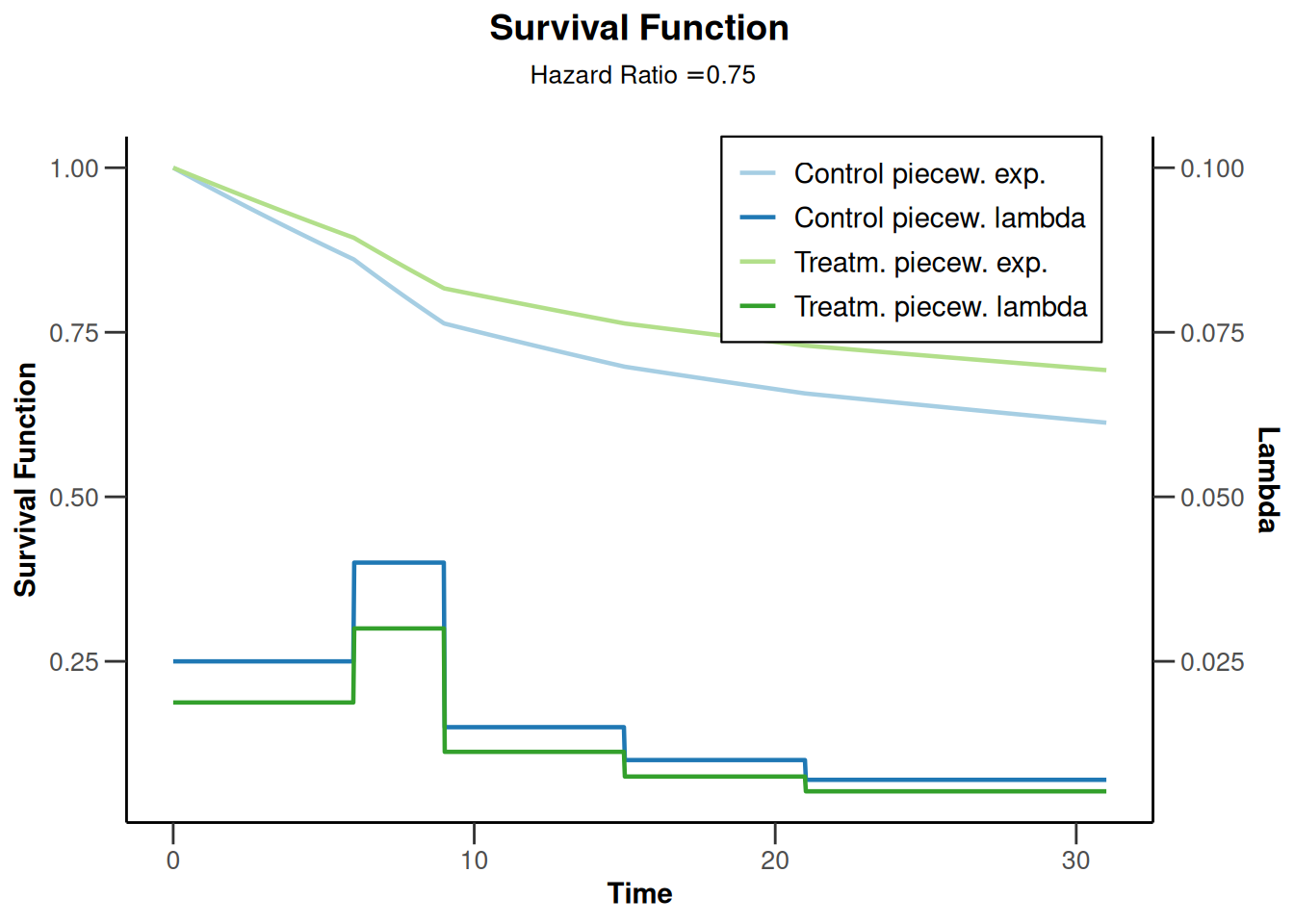

Power calculation

The function getPowerSurvival() is the analogue of getSampleSizeSurvival() for power calculations and has a very similar syntax. We illustrate its usage for the above example below.

Example - piece-wise exponential survival, constant accrual intensity, group sequential design (continued)

What is the power of the trial from the example above if the true hazard ratio is 0.7 rather than the targeted hazard ratio of 0.75 above?

The corresponding power calculation is given below. The function call uses the same arguments as the call to function getSampleSizeSurvival() above except that the maximum sample size of 1000 and the maximum number of events of 387 from above are provided as arguments and the hazard ratio is changed to 0.7. In addition, the direction of the test (directionUpper) needs to be specified.

powerResult <- getPowerSurvival(
    design = design,
    piecewiseSurvivalTime = piecewiseSurvivalTime, 
    hazardRatio = 0.7,
    dropoutRate1 = 0.05, 
    dropoutRate2 = 0.05, 
    dropoutTime = 12,
    accrualTime = 0, 
    accrualIntensity = 42,
    maxNumberOfSubjects = 1000, 
    maxNumberOfEvents = 387, 
    directionUpper = FALSE
)
powerResult

Design plan parameters and output for survival data

Design parameters

Information rates: 0.500, 0.750, 1.000
Critical values: 2.963, 2.359, 2.014
Futility bounds (non-binding): -Inf, -Inf
Cumulative alpha spending: 0.001525, 0.009649, 0.025000
Local one-sided significance levels: 0.001525, 0.009162, 0.022000
Significance level: 0.0250
Test: one-sided

User defined parameters

Direction upper: FALSE
Piecewise survival lambda (2): 0.025, 0.040, 0.015, 0.010, 0.007
Hazard ratio: 0.700
Maximum number of subjects: 1000
Maximum number of events: 387
Accrual time: 23.81
Accrual intensity: 42.0
Piecewise survival times: 0.00, 6.00, 9.00, 15.00, 21.00
Drop-out rate (1): 0.050
Drop-out rate (2): 0.050

Default parameters

Theta H0: 1
Type of computation: Schoenfeld
Planned allocation ratio: 1
kappa: 1
Drop-out time: 12.00

Power and output

Piecewise survival lambda (1): 0.0175, 0.0280, 0.0105, 0.0070, 0.0049
Number of subjects [1]: 990.4
Number of subjects [2]: 1000
Number of subjects [3]: 1000
Follow up time: 39.56
Expected number of events: 283.6
Overall reject: 0.9355
Reject per stage [1]: 0.3150
Reject per stage [2]: 0.4392
Reject per stage [3]: 0.1813
Early stop: 0.7542
Analysis time [1]: 23.58
Analysis time [2]: 34.72
Analysis time [3]: 63.37
Expected study duration: 38.26
Maximal study duration: 63.37
Cumulative number of events [1]: 193.5
Cumulative number of events [2]: 290.2
Cumulative number of events [3]: 387
Expected number of subjects: 997
Critical values (treatment effect scale) [1]: 0.653
Critical values (treatment effect scale) [2]: 0.758
Critical values (treatment effect scale) [3]: 0.815

Legend

(i): values of treatment arm i
[k]: values at stage k

This yields an overall power of 0.935. Note also that the timing of the interim analyses is slightly deferred now (as the events now occur more slowly in the intervention arm) but the expected study duration is decreased from 43.87 to 38.26 months because chances to stop the trial early have increased.

The impact of the true hazard ratio on power and study duration can also be calculated by entering the hazardRatio argument as a vector. Below, the hazard ratio is varied from 0.6 to 1 (in increments of 0.02) and the results are displayed graphically.

powerResult2 <- getPowerSurvival(
    design = design,
    piecewiseSurvivalTime = piecewiseSurvivalTime, 
    hazardRatio = seq(0.6, 1, by = 0.02),
    dropoutRate1 = 0.05, 
    dropoutRate2 = 0.05, 
    dropoutTime = 12,
    accrualTime = 0, 
    accrualIntensity = 42,
    maxNumberOfSubjects = 1000, 
    maxNumberOfEvents = 387, 
    directionUpper = FALSE
)

# Plot true hazard ratio vs overall power, probability of an early rejection,
# and expected number of events
powerResult2 |> plot(type = 6, legendPosition = 3) # legend in left bottom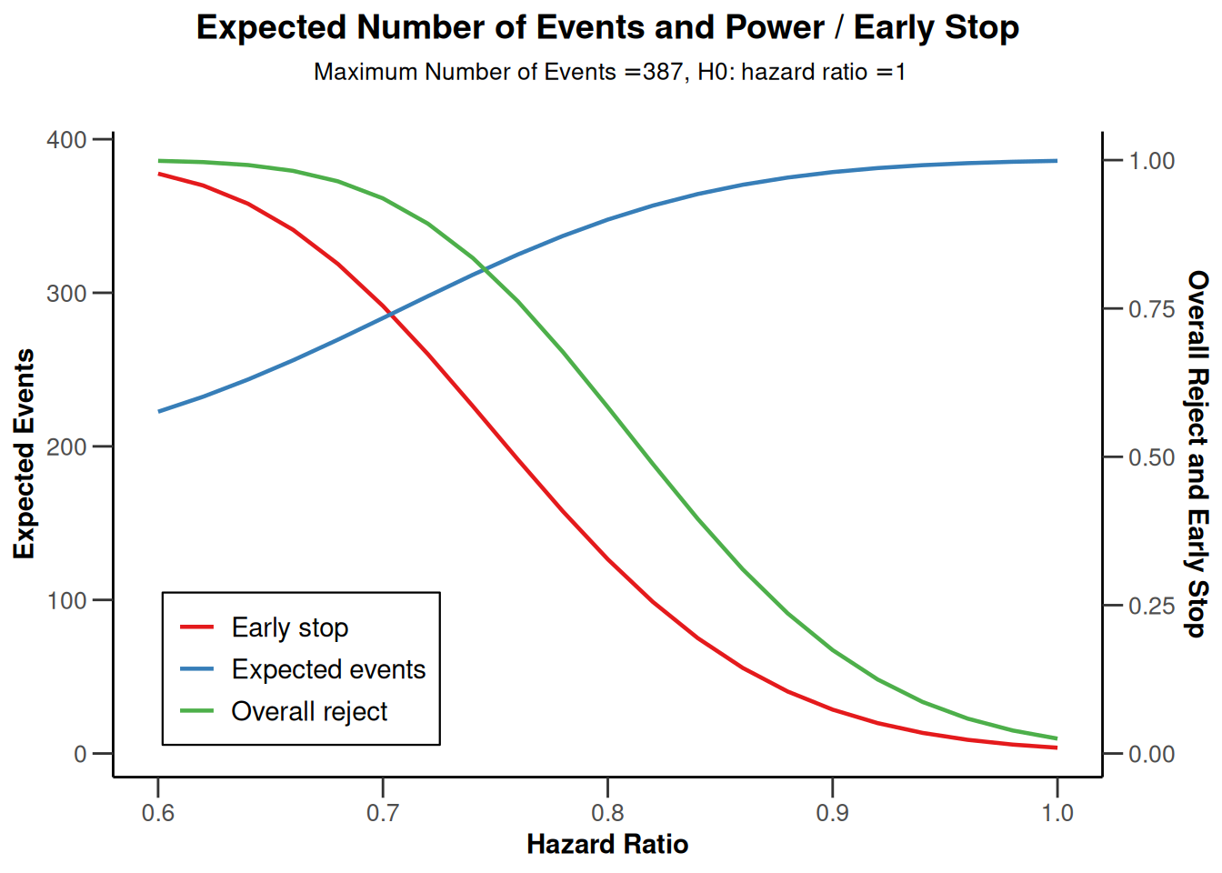

# Plot hazard ratio vs analysis time
powerResult2 |> plot(type = 12, legendPosition = 4) # right top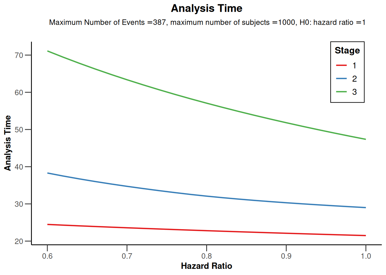

For examples of all available plots in rpact, see the R vignette How to create admirable plots with rpact).

Prediction of number of events over time

The function getEventProbabilities calculates the probability that a randomly chosen subject has an observed event up to a specied time after the start of the study. By multiplying this probability with the maximal sample size, we obtain the expected number of events up to that time point.

The arguments for the function getEventProbabilities are similar to those for the function getSampleSizeSurvival discussed above. One difference is that the maximal sample size must always be provided in function getEventProbabilities. This can either be done explicitly by setting argument maxNumberOfSubjects or implicitly by specifying the accrual duration as described in Section @ref(accrualDurationKnown).

For illustration, we revisit the example from Section @ref(sampleSizeGroupSeq). In that example, the sample size was 1000 and the expected timing of the final analysis after observing 387 events was after 60.00 months. The code below re-calculates the expected number of events until that time point.

# Sample size per arm and overall for the example
maxNumberOfSubjects1 <- 500
maxNumberOfSubjects2 <- 500
maxNumberOfSubjects <- maxNumberOfSubjects1 + maxNumberOfSubjects2

# Probability that a randomly chosen subject has an observed event
# until 60 months after study start
probEvent <- getEventProbabilities(
    time = 60,
    piecewiseSurvivalTime = piecewiseSurvivalTime, 
    hazardRatio = 0.75,
    dropoutRate1 = 0.05, 
    dropoutRate2 = 0.05, 
    dropoutTime = 12,
    accrualTime = 0, 
    accrualIntensity = 42,
    maxNumberOfSubjects = maxNumberOfSubjects
)
probEvent

Event probabilities at given time

User defined parameters

Time: 60.00
Accrual time: 23.81
Accrual intensity: 42.0
Piecewise survival times: 0.00, 6.00, 9.00, 15.00, 21.00
lambda(2): 0.025, 0.040, 0.015, 0.010, 0.007
Hazard ratio: 0.750
Drop-out rate (1): 0.050
Drop-out rate (2): 0.050
Maximum number of subjects: 1000

Default parameters

kappa: 1
Planned allocation ratio: 1
Drop-out time: 12.00

Time and output

lambda(1): 0.01875, 0.03000, 0.01125, 0.00750, 0.00525
Cumulative event probabilities: 0.3868
Event probabilities (1): 0.3444
Event probabilities (2): 0.4292

Legend

(i): values of treatment arm i

# Total expected number of events until 60 months
probEvent$cumulativeEventProbabilities * maxNumberOfSubjects

[1] 386.7958

# Expected number of events per group until 60 months
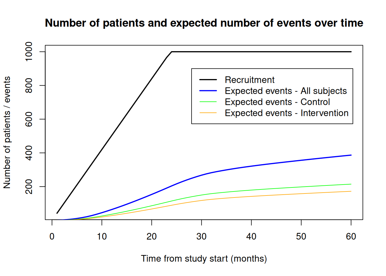
probEvent$eventProbabilities1 * maxNumberOfSubjects1 # intervention

[1] 172.1793

probEvent$eventProbabilities2 * maxNumberOfSubjects2 # control

[1] 214.6165

The function getEventProbabilities() also allows a vector argument for time and the code below illustrates how to calculate (and plot) expected event numbers over time (overall and by group). In addition, the number of recruited subjects is added to the plot which can be obtained with function getNumberOfSubjects().

time <- 1:60

# Expected number of events overall and per group at 1-60 months after study start
probEvent <- getEventProbabilities(
    time = time,
    piecewiseSurvivalTime = piecewiseSurvivalTime, 
    hazardRatio = 0.75,
    dropoutRate1 = 0.05, 
    dropoutRate2 = 0.05, 
    dropoutTime = 12,
    accrualTime = 0, 
    accrualIntensity = 42,
    maxNumberOfSubjects = maxNumberOfSubjects
)
expEvent <- probEvent$cumulativeEventProbabilities * maxNumberOfSubjects # overall
expEventInterv <- probEvent$eventProbabilities1 * maxNumberOfSubjects1 # intervention
expEventCtrl <- probEvent$eventProbabilities2 * maxNumberOfSubjects2 # control

# Cumulative number of recruited patients over time
nSubjects <- getNumberOfSubjects(
    time = time, 
    accrualTime = 0,
    accrualIntensity = 42, 
    maxNumberOfSubjects = maxNumberOfSubjects
)
# plot result
plot(time, nSubjects$numberOfSubjects,
    type = "l", lwd = 2,
    main = "Number of patients and expected number of events over time",
    xlab = "Time from study start (months)",
    ylab = "Number of patients / events"
)
lines(time, expEvent, col = "blue", lwd = 2)
lines(time, expEventCtrl, col = "green")
lines(time, expEventInterv, col = "orange")
legend(
    x = 28, y = 900,
    legend = c(
        "Recruitment", "Expected events - All subjects",
        "Expected events - Control", "Expected events - Intervention"
    ),
    col = c("black", "blue", "green", "orange"), lty = 1, lwd = c(2, 2, 1, 1)
)

Interim analyses for multiple time-to-event endpoints

The function getEventProbabilities() can also be used to align interim analyses of different time to event endpoints as illustrated in two examples below.

Example: Both PFS and OS as primary endpoints, OS interim aligned with PFS final analysis

Overall Type I error 5% (two-sided), 1:1 randomized with PFS and OS both as primary endpoints.
Assumptions for PFS (1% Type I error assigned):
- Median PFS control is 6 months, target hazard ratio is 0.65, 95% power at two-sided 1% significance level.
- Only one primary analysis.
Assumptions for OS (4% Type I error assigned):
- Median OS control is 12 month, target hazard ratio is 0.75, 80% power at two-sided 4% significance level.
- Interim analysis at the primary PFS analysis, final analysis when the target number of OS events has been reached.
- O’Brien & Fleming type $\alpha$-spending function.
Uniform recruitment of 60 patients/month over 10 months, no dropout.

To display results more concisely, all outputs below were created with the generic summary() function.

The first step is to calculate the required number of events and the timing of the primary analyses for PFS:

sampleSizePFS <- getSampleSizeSurvival(
    beta = 0.05, 
    sided = 2, 
    alpha = 0.01,
    lambda2 = log(2) / 6, 
    hazardRatio = 0.65,
    accrualTime = c(0, 10), 
    accrualIntensity = 60
)
sampleSizePFS |> summary()

Sample size calculation for a survival endpoint

Fixed sample analysis, two-sided significance level 1%, power 95%. The results were calculated for a two-sample logrank test, H0: hazard ratio = 1, H1: hazard ratio = 0.65, control lambda(2) = 0.116, accrual time = 10, accrual intensity = 60.

Stage	Fixed
Stage level (two-sided)	0.0100
Efficacy boundary (z-value scale)	2.576
Lower efficacy boundary (t)	0.769
Upper efficacy boundary (t)	1.301
Number of subjects	600.0
Number of events	384.0
Analysis time	16.37
Expected study duration under H1	16.37

Legend:

(t): treatment effect scale

Based on this, the estimated time of the primary PFS analysis is after 16.37 months.

Second, we calculate the expected number of OS events at the final PFS analysis after 16.37 months.

# Expected number of OS events at the time of the final PFS analysis
probOS <- getEventProbabilities(
    time = 16.37,
    accrualTime = c(0, 10), 
    accrualIntensity = 60,
    lambda2 = log(2) / 12, 
    hazardRatio = 0.75
)
probOS$cumulativeEventProbabilities * 600

[1] 257.5158

Third, we calculate the required number of events and the timing of analyses for OS using an initial guess for the information fraction at the OS interim analysis of 50%:

# Preliminary group sequential design for OS assuming interim at 50% information
designOS1 <- getDesignGroupSequential(
    sided = 2, 
    alpha = 0.04, 
    beta = 0.2,
    informationRates = c(0.5, 1), 
    typeOfDesign = "asOF"
)
# Preliminary sample size for OS assuming interim at 50% information
sampleSizeOS1 <- getSampleSizeSurvival(
  designOS1,
  lambda2 = log(2) / 12, 
  hazardRatio = 0.75,
  accrualTime = c(0, 10), 
  accrualIntensity = 60
)
sampleSizeOS1 |> summary()

Sample size calculation for a survival endpoint

Sequential analysis with a maximum of 2 looks (group sequential design), two-sided overall significance level 4%, power 80%. The results were calculated for a two-sample logrank test, H0: hazard ratio = 1, H1: hazard ratio = 0.75, control lambda(2) = 0.058, accrual time = 10, accrual intensity = 60.

Stage	1	2
Planned information rate	50%	100%
Cumulative alpha spent	0.0020	0.0400
Stage levels (two-sided)	0.0020	0.0393
Efficacy boundary (z-value scale)	3.090	2.061
Lower efficacy boundary (t)	0.648	0.815
Upper efficacy boundary (t)	1.543	1.227
Cumulative power	0.1493	0.8000
Number of subjects	600.0	600.0
Expected number of subjects under H1		600.0
Cumulative number of events	203.2	406.4
Expected number of events under H1		376.0
Analysis time	13.43	27.85
Expected study duration under H1		25.70
Exit probability for efficacy (under H0)	0.0020
Exit probability for efficacy (under H1)	0.1493

Legend:

(t): treatment effect scale

Finally, we recalculate the required number of events and timing of analyses for OS using an updated estimate of the information fraction at the interim analysis. Specifically, we calculate this fraction as the expected number of events at the time of the final PFS analysis (i.e., 258 events) relative to the maximal number of events based on the calculation for OS above (i.e., 407):

# Updated group sequential design for OS assuming an updated information fraction
designOS2 <- getDesignGroupSequential(
  sided = 2, 
  alpha = 0.04, 
  beta = 0.2,
  informationRates = c(258 / 407, 1), 
  typeOfDesign = "asOF"
)
# Updated sample size for OS
sampleSizeOS2 <- getSampleSizeSurvival(
  designOS2,
  lambda2 = log(2) / 12, 
  hazardRatio = 0.75,
  accrualTime = c(0, 10), 
  accrualIntensity = 60
)
sampleSizeOS2 |> summary()

Sample size calculation for a survival endpoint

Stage	1	2
Planned information rate	63.4%	100%
Cumulative alpha spent	0.0070	0.0400
Stage levels (two-sided)	0.0070	0.0378
Efficacy boundary (z-value scale)	2.699	2.077
Lower efficacy boundary (t)	0.715	0.814
Upper efficacy boundary (t)	1.398	1.228
Cumulative power	0.3508	0.8000
Number of subjects	600.0	600.0
Expected number of subjects under H1		600.0
Cumulative number of events	259.2	408.8
Expected number of events under H1		356.3
Analysis time	16.47	28.11
Expected study duration under H1		24.03
Exit probability for efficacy (under H0)	0.0070
Exit probability for efficacy (under H1)	0.3508

Legend:

(t): treatment effect scale

According to the updated calculation, the panned timing of the OS interim analysis is after 16.47 months which is sufficiently close to the planned timing of the PFS final analysis after 16.37 months for planning purposes.

Example: Power considerations for OS as a secondary endpoint, OS interim aligned with primary PFS analysis

Overall Type I error 5% (two-sided), 1:1 randomized with PFS as the primary endpoint.
Sample size calculation for PFS resulted in the following design:
- No interim analyses for PFS.
- Uniform recruitment of 80 patients/month over 10 months (800 patients in total), no dropout.
- Final PFS analysis with 80% power for the targeted HR is expected after a study duration of 24 months.
Asssumption for OS:
- Median OS 30 months, OS HR expected to be around 0.8.
- OS is only formally tested if PFS is significant (hierarchical testing).
- One interim analysis at the time of the final PFS analysis.
- It is anticipated that the OS analysis cannot be fully powered. The target number of OS events at the final OS analysis will be pre-defined after considering all possible trade-offs between study power and duration.
- O’Brien & Fleming type $\alpha$-spending function.

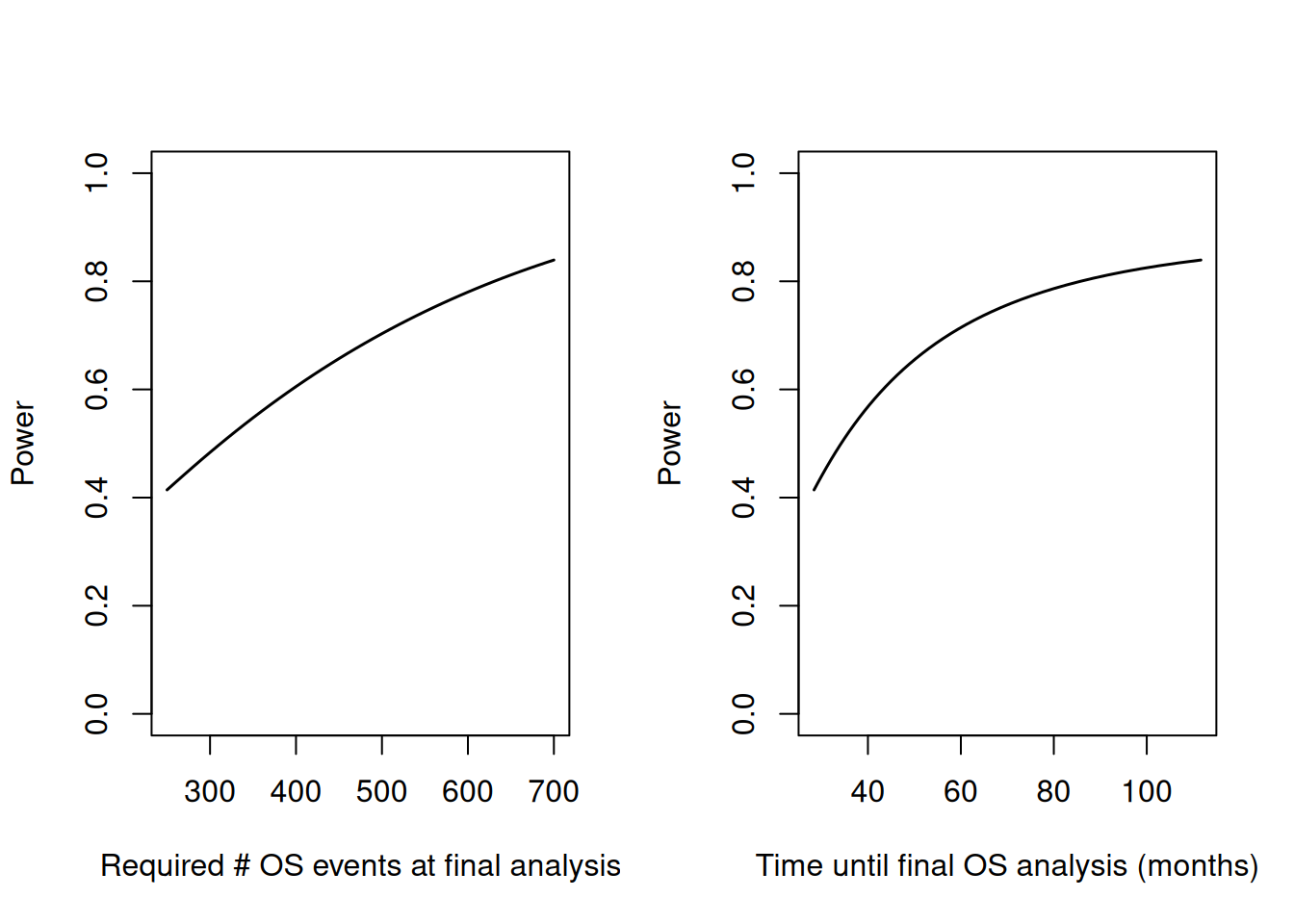
The code below calulates study duration and power for the final OS analysis (conditional on significance for the primary PFS analysis) depending on the target number of OS events at the final analysis. The resulting plots should facilitate the final choice of the timing of the OS analysis.

# 1) Calculate expected number of OS events at the time of the final PFS analysis
noDeathsAtPFSAnalysis <- getEventProbabilities(
    time = 24,
    lambda2 = log(2) / 30, 
    hazardRatio = 0.8,
    accrualTime = c(0, 20), 
    accrualIntensity = 40
)$cumulativeEventProbabilities * 800
noDeathsAtPFSAnalysis

[1] 197.4038

# 2) Set up data frame which will contain number of OS events and
#    corresponding power and study durations
#    (vary target number of OS events from 250-700)
powerOSevents <- data.frame(
    maxNumberOSEvents = seq(250, 700, by = 10),
    power = NA,
    durationFinalOSAnalysis = NA
)

# 3) Calculate power and study durations depending on target number of OS events
for (i in 1:nrow(powerOSevents)) {
    # Define OF-type design, with first interim after noDeathsAtPFSAnalysis events
    # and final analysis after maxNumberOSEvents[i] events
    # PS: beta not explicitly set here because boundary and
    #     subsequent power calculations do not depend on it
    informationRates <- c(noDeathsAtPFSAnalysis, powerOSevents$maxNumberOSEvents[i]) /
        powerOSevents$maxNumberOSEvents[i]
    design <- getDesignGroupSequential(
        sided = 2, 
        alpha = 0.05, 
        typeOfDesign = "asOF",
        informationRates = informationRates, 
        twoSidedPower = TRUE
    )
    # Power and study duration after maxNumberOSEvents[i]
    powerResult <- getPowerSurvival(
        design = design,
        lambda2 = log(2) / 30, 
        hazardRatio = 0.8,
        accrualTime = c(0, 20), 
        accrualIntensity = 40,
        maxNumberOfEvents = powerOSevents$maxNumberOSEvents[i]
    )
    powerOSevents$power[i] <- powerResult$overallReject
    powerOSevents$durationFinalOSAnalysis[i] <- powerResult$maxStudyDuration
}

# 4) Plot results
par(mfrow = c(1, 2))
#  events cs power
plot(powerOSevents$maxNumberOSEvents,
    powerOSevents$power,
    type = "l",
    xlab = "Required # OS events at final analysis",
    ylab = "Power", 
    ylim = c(0, 1), 
    lwd = 1.5
)
# Duration vs power
plot(powerOSevents$durationFinalOSAnalysis,
    powerOSevents$power,
    type = "l",
    xlab = "Time until final OS analysis (months)",
    ylab = "Power", 
    ylim = c(0, 1), 
    lwd = 1.5
)

Extracting information from rpact objects

names(rpact_object) gives variable names of an rpact object which can be accessed via rpact_object$varname. For example, sampleSizeResult$studyDurationH1 contains the expected study duration under H1. For more details on using R generics for rpact objects, please refer to vignette Example: using rpact with R generics.

System: rpact 4.1.1, R version 4.4.2 (2024-10-31 ucrt), platform: x86_64-w64-mingw32

To cite R in publications use:

R Core Team (2024). R: A Language and Environment for Statistical Computing. R Foundation for Statistical Computing, Vienna, Austria. https://www.R-project.org/.

To cite package ‘rpact’ in publications use:

Wassmer G, Pahlke F (2024). rpact: Confirmatory Adaptive Clinical Trial Design and Analysis. R package version 4.1.1, https://www.rpact.com, https://github.com/rpact-com/rpact, https://rpact-com.github.io/rpact/, https://www.rpact.org.

Reuse

CC BY-SA 4.0

Designing Group Sequential Trials with Two Groups and a Survival Endpoint with rpact

Introduction

Overview of relevant rpact functions

Specifying survival distributions in rpact

Exponential survival distributions

Event probability at a specific time point known

Exponential parameter \(\lambda\) known

Median survival known

Weibull

Piecewise exponential survival

Piecewise constant hazard rate \(\lambda\) in each interval known

Survival function at different time points known

Appendix: Random numbers, cumulative distribution, and quantiles for the piecewise exponential distribution

Specifying dropout in rpact

Specifying accrual in rpact

Absolute accrual intensity and accrual duration known

Absolute accrual intensity known, accrual duration unknown

Sample size calculation for superiority trials without interim analyses

Example - exponential survival, flexible accrual intensity, no interim analyses

Sample size calculation for non-inferiority trials without interim analyses

Sample size calculation for trials with interim analyses

Example - piece-wise exponential survival, constant accrual intensity, group sequential design

Sample size calculation

Sample size plots

Power calculation

Example - piece-wise exponential survival, constant accrual intensity, group sequential design (continued)

Prediction of number of events over time

Interim analyses for multiple time-to-event endpoints

Example: Both PFS and OS as primary endpoints, OS interim aligned with PFS final analysis

Example: Power considerations for OS as a secondary endpoint, OS interim aligned with primary PFS analysis

Extracting information from rpact objects

Reuse