Simulation of a Trial with a Binary Endpoint and Unblinded Sample Size Re-Calculation with rpact
Planning
Rates
Sample size
Power simulation
This document provides examples for assessing trials with adaptive sample size re-calculation (SSR) using rpact. It also shows how to implement the promising zone approach as proposed by Mehta and Pocock (2011) and further developed by Hsiao et al. (2019) with rpact.
rpact provides the functions getSimulationMeans() (continuous endpoints), getSimulationRates() (binary endpoints) and getSimulationSurvival() (time-to-event endpoints) for simulation of group sequential trials with adaptive SSR.
For trials with adaptive SSR, the design can be created with the functions getDesignInverseNormal() or getDesignFisher(). The sample size is re-calculated based on the target conditional power (argument conditionalPower). Conditional power is by default evaluated at the observed estimates for the parameters. If the evaluation of conditional power at other parameter values is desired, they can be provided as arguments thetaH1 (for getSimulationMeans() and getSimulationSurvival()), or pi1H1 and pi2H1 (for getSimulationRates()). For continuous endpoints, by default, conditional power is evaluated at the standard deviation stDev under which the trial is simulated. In rpact 3.0, a variable stDevH1 can be entered to specify the standard deviation that is used for the sample size recalculation.
For the functions getSimulationMeans() and getSimulationRates() (but not in getSimulationSurvival()), the SSR function can be optionally modified using the argument calcSubjectsFunction() (see the respective help pages and the code below for details and examples).
In this vignette, we present an example of the use of these functions for a trial with a binary endpoint. For this, we will use the constraint promizing zone approach as described in Hsiao et al. (2019).
For this vignette, additionally to rpact itself and ggplot2, we use the packages ggpubr and dplyr.
Assumptions and design options
1:1 randomized superiority trial with overall response rate (ORR) as the primary endpoint (binary)
ORR in the control arm is known to be ~20%
The novel treatment may increase ORR by 10%-13%
2.5% one-sided significance level
We first calculate the sample sizes (per treatment group) for the corresponding fixed designs with 90% power:
# fixed design powered for delta of 13%ssMin <-getSampleSizeRates(pi1 =0.33, pi2 =0.2, alpha =0.025, beta =0.1)(Nmin <-ceiling(ssMin$numberOfSubjects1))
     [,1]
[1,]  241
# fixed design powered for delta of 10%ssMax <-getSampleSizeRates(pi1 =0.30, pi2 =0.2, alpha =0.025, beta =0.1)(Nmax <-ceiling(ssMax$numberOfSubjects1))
     [,1]
[1,]  392
Assume that the sponsor is unwilling to make an up-front commitment for a trial with Nmax = 392 subjects per treatment group but that they are willing to provide an up-front commitment for a trial with Nmin = 241 subjects per treatment group. If the results at an interim analysis with an unblinded SSR look “promising”, the sponsor would then be willing to commit funding for up to 392 subjects per treatment group in total.
To help the sponsor, we investigate two designs with an interim analysis for SSR after 120 subjects per treatment group:
SSR based on conditional power: adjust sample size to achieve a conditional power of 90% assuming that the true response rates are 20% and 30% (if this is feasible within the given sample size range)
A constrained promising zone design (Hsiao et al., 2019) with \(cp_{min} = 80\%\) and \(cp_{max} = 90\%\).
To combine the two stages for both designs, we use an inverse normal combination test with optimal weights for the minimal final group size (practically, this is a design with equal weights) and no provision for early stopping for neither efficacy nor futility at interim:
# group size at interimn1 <-floor(Nmin /2)
# inverse normal design with possible rejection of H0 only at the final analysisdesignIN <-getDesignInverseNormal(typeOfDesign ="noEarlyEfficacy",kMax =2,alpha =0.025)designIN |>summary()
Sequential analysis with a maximum of 2 looks (inverse normal combination test design)
No early efficacy stop design, one-sided overall significance level 2.5%, undefined endpoint.
Stage
1
2
Fixed weight
0.707
0.707
Cumulative alpha spent
0
0.0250
Stage levels (one-sided)
0
0.0250
Efficacy boundary (z-value scale)
Inf
1.960
Design with SSR (SSR) based on conditional power
It is straightforward to simulate the test characteristics from this design using the function getSimulationRates(). plannedSubjects refers to the cumulated sample sizes over the two stages in both treatment groups. If conditionalPower is specified, minNumberOfSubjectsPerStage and maxNumberOfSubjectsPerStage must be specified. They refer to the minimum and maximum overall sample sizes per stage (the first element is the first stage sample size), respectively. If pi1H1 and/or pi2H1 are not specified, the observed (simulated) rates at interim are used for the SSR.
# Design with sample size re-estimated to get conditional power of 0.9 at# pi1H1 = 0.3, pi2H1 = 0.2 [minimum effect size]# (evaluate at most interesting values for pi1)simCpower <-getSimulationRates(designIN,pi1 =c(0.2, 0.3, 0.33), pi2 =0.2,# cumulative overall sample sizeplannedSubjects =2*c(n1, Nmin),conditionalPower =0.9,# stage-wise minimal overall sample sizeminNumberOfSubjectsPerStage =2*c(n1, (Nmin - n1)),# stage-wise maximal overall sample sizemaxNumberOfSubjectsPerStage =2*c(n1, (Nmax - n1)),pi1H1 =0.3, pi2H1 =0.2,maxNumberOfIterations =1000,seed =12345,showStatistics =FALSE)simCpower
Simulation of rates (inverse normal combination test design)
Design parameters
Information rates: 0.500, 1.000
Critical values: Inf, 1.960
Futility bounds (non-binding): -Inf
Cumulative alpha spending: 0.0000, 0.0250
Local one-sided significance levels: 0.0000, 0.0250
Significance level: 0.0250
Test: one-sided
User defined parameters
Seed: 12345
Conditional power: 0.9
Planned cumulative subjects: 240, 482
Minimum number of subjects per stage: 240, 242
Maximum number of subjects per stage: 240, 544
Assumed treatment rate: 0.200, 0.300, 0.330
pi(1) under H1: 0.300
Assumed control rate: 0.200
Default parameters
Maximum number of iterations: 1000
Planned allocation ratio: 1
Direction upper: TRUE
Treatment groups: 2
Normal approximation: TRUE
pi(2) under H1: 0.200
Risk ratio: FALSE
Theta H0: 0
Results
Effect: 0.00, 0.10, 0.13
Iterations [1]: 1000, 1000, 1000
Iterations [2]: 1000, 1000, 1000
Overall reject: 0.0220, 0.8590, 0.9730
Reject per stage [1]: 0.0000, 0.0000, 0.0000
Reject per stage [2]: 0.0220, 0.8590, 0.9730
Overall futility stop: 0.0000, 0.0000, 0.0000
Futility stop per stage: 0.0000, 0.0000, 0.0000
Early stop: 0.0000, 0.0000, 0.0000
Expected number of subjects: 771.7, 631.5, 577.2
Sample sizes [1]: 240, 240, 240
Sample sizes [2]: 531.7, 391.5, 337.2
Conditional power (achieved) [1]: NA, NA, NA
Conditional power (achieved) [2]: 0.4821, 0.8579, 0.9092
Legend
(i): values of treatment arm i
[k]: values at stage k
Constrained promising zone (CPZ) design
As described in Hsiao et al. (2019), this method chooses the sample size according to the following rules:
Choose the second stage sample size \(N^*\) between \(Nmin\) and \(Nmax\) such that the conditional power is \(cp_{max}\) for the minimal effect size we want to detect (i.e., ORR of 20% vs. 30%). We choose \(cp_{max} = 0.90\) here as in the original publication.
If such a sample size \(N^*\) does not exist, then proceed as follows:
If the conditional power cannot be boosted to at least \(cp_{min}\) by increasing the sample size to \(Nmax\), i.e., if the interim result is not considered «promising», then do not increase the sample and set \(N^* = Nmin\). We choose \(cp_{min} = 0.80\) here as in the original publication.
Otherwise: set \(N^* = Nmax\)
To simulate the CPZ design in rpact, we can use the function getSimulationRates() again. However, the situation is more complicated because we need to re-define the sample size recalculation rule using the argument calcSubjectsFunction (see the help page ?getSimulationRates for more information regarding calcSubjectsFunction()):
# CPZ design (evaluate at the most interesting values for pi1)# home-made SSR functionmyCPZSampleSizeCalculationFunction <-function(..., stage, plannedSubjects, conditionalPower, minNumberOfSubjectsPerStage, maxNumberOfSubjectsPerStage, conditionalCriticalValue, overallRate) { rateUnderH0 <- (overallRate[1] + overallRate[2]) /2# function adapted from example in ?getSimulationRates calculateStageSubjects <-function(cp) {2* (max(0, conditionalCriticalValue *sqrt(2* rateUnderH0 * (1- rateUnderH0)) + stats::qnorm(cp) *sqrt(overallRate[1] * (1- overallRate[1]) + overallRate[2] * (1- overallRate[2]))))^2/ (max(1e-12, (overallRate[1] - overallRate[2])))^2 }# Calculate sample size required to reach maximum desired conditional power# cp_max (provided as argument conditionalPower) stageSubjectsCPmax <-calculateStageSubjects(cp = conditionalPower)# Calculate sample size required to reach minimum desired conditional power# cp_min (**manually set for this example to 0.8**) stageSubjectsCPmin <-calculateStageSubjects(cp =0.8)# Define stageSubjects stageSubjects <-ceiling(min(max( minNumberOfSubjectsPerStage[stage], stageSubjectsCPmax ), maxNumberOfSubjectsPerStage[stage]))# Set stageSubjects to minimal sample size in case minimum conditional power# cannot be reached with available sample sizeif (stageSubjectsCPmin > maxNumberOfSubjectsPerStage[stage]) { stageSubjects <- minNumberOfSubjectsPerStage[stage] }# return sample sizereturn(stageSubjects)}# Now simulate the CPZ designsimCPZ <-getSimulationRates(designIN,pi1 =c(0.2, 0.3, 0.33), pi2 =0.2,plannedSubjects =2*c(n1, Nmin), # cumulative overall sample sizeconditionalPower =0.9,# stage-wise minimal overall sample sizeminNumberOfSubjectsPerStage =2*c(n1, (Nmin - n1)),# stage-wise maximal overall sample sizemaxNumberOfSubjectsPerStage =2*c(n1, (Nmax - n1)),pi1H1 =0.3, pi2H1 =0.2,calcSubjectsFunction = myCPZSampleSizeCalculationFunction,maxNumberOfIterations =1000,seed =12345, showStatistics =FALSE)simCPZ
Simulation of rates (inverse normal combination test design)
Design parameters
Information rates: 0.500, 1.000
Critical values: Inf, 1.960
Futility bounds (non-binding): -Inf
Cumulative alpha spending: 0.0000, 0.0250
Local one-sided significance levels: 0.0000, 0.0250
Significance level: 0.0250
Test: one-sided
User defined parameters
Seed: 12345
Conditional power: 0.9
Planned cumulative subjects: 240, 482
Minimum number of subjects per stage: 240, 242
Maximum number of subjects per stage: 240, 544
Calculate subjects function: user defined
Assumed treatment rate: 0.200, 0.300, 0.330
pi(1) under H1: 0.300
Assumed control rate: 0.200
Default parameters
Maximum number of iterations: 1000
Planned allocation ratio: 1
Direction upper: TRUE
Treatment groups: 2
Normal approximation: TRUE
pi(2) under H1: 0.200
Risk ratio: FALSE
Theta H0: 0
Results
Effect: 0.00, 0.10, 0.13
Iterations [1]: 1000, 1000, 1000
Iterations [2]: 1000, 1000, 1000
Overall reject: 0.0190, 0.8070, 0.9460
Reject per stage [1]: 0.0000, 0.0000, 0.0000
Reject per stage [2]: 0.0190, 0.8070, 0.9460
Overall futility stop: 0.0000, 0.0000, 0.0000
Futility stop per stage: 0.0000, 0.0000, 0.0000
Early stop: 0.0000, 0.0000, 0.0000
Expected number of subjects: 525.7, 574.5, 550.1
Sample sizes [1]: 240, 240, 240
Sample sizes [2]: 285.7, 334.5, 310.1
Conditional power (achieved) [1]: NA, NA, NA
Conditional power (achieved) [2]: 0.2827, 0.7883, 0.8898
Legend
(i): values of treatment arm i
[k]: values at stage k
Graphical comparison of the two designs
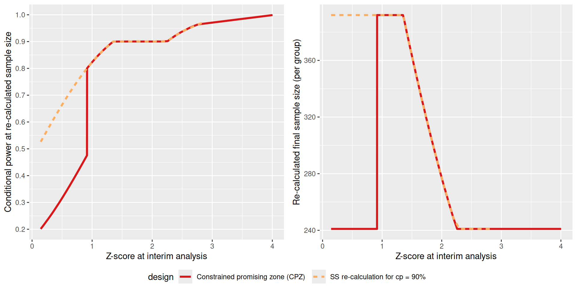
We first use the aggregated data from the two simulations to compare the dependence of the re-calculated sample size and the corresponding conditional power on the interim Z-score between the two designs. For this, we use the function getData(), the summarize() command of the dplyr package and plot it with ggplot2. Note that for this illustration we summarize over all values of pi1. This makes sense because we used a fixed pi1H1 and pi2H1 for both sample size simulation methods.
# aggregate data across simulation runs for both simulations and extract Z-score,# conditionalPower, and totalSampleSize1 (per group)aggSimCpower <-getData(simCpower)sumCpower <- aggSimCpower %>%group_by(iterationNumber) %>%summarise(design ="SS re-calculation for cp = 90%",Z1 = testStatistic[1], conditionalPower = conditionalPowerAchieved[2],totalSampleSize1 = (numberOfSubjects[1] + numberOfSubjects[2]) /2 ) %>%arrange(Z1) %>%filter(Z1 >0, Z1 <5)aggSimCPZ <-getData(simCPZ)sumCPZ <- aggSimCPZ %>%group_by(iterationNumber) %>%summarise(design ="Constrained promising zone (CPZ)",Z1 = testStatistic[1], conditionalPower = conditionalPowerAchieved[2],totalSampleSize1 = (numberOfSubjects[1] + numberOfSubjects[2]) /2 ) %>%arrange(Z1) %>%filter(Z1 >0, Z1 <5)sumBoth <-rbind(sumCpower, sumCPZ)# Plot itplot1 <-ggplot(aes(Z1, conditionalPower,col = design,group = design), data = sumBoth) +geom_line(aes(linetype = design), lwd =1.2) +scale_x_continuous(name ="Z-score at interim analysis") +scale_y_continuous(breaks =seq(0, 1, by =0.1),name ="Conditional power at re-calculated sample size" ) +scale_color_manual(values =c("#d7191c", "#fdae61"))plot2 <-ggplot(aes(Z1, totalSampleSize1,col = design,group = design), data = sumBoth) +geom_line(aes(linetype = design), lwd =1.2) +scale_x_continuous(name ="Z-score at interim analysis") +scale_y_continuous(name ="Re-calculated final sample size (per group)") +scale_color_manual(values =c("#d7191c", "#fdae61"))ggarrange(plot1, plot2, common.legend =TRUE, legend ="bottom")
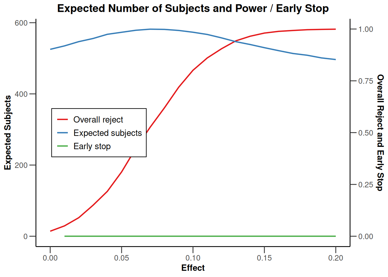
To compare the two designs across a wider range of parameters, we re-simulate the designs for a finer grid of assumed ORR in the intervention group and then visualize the results.
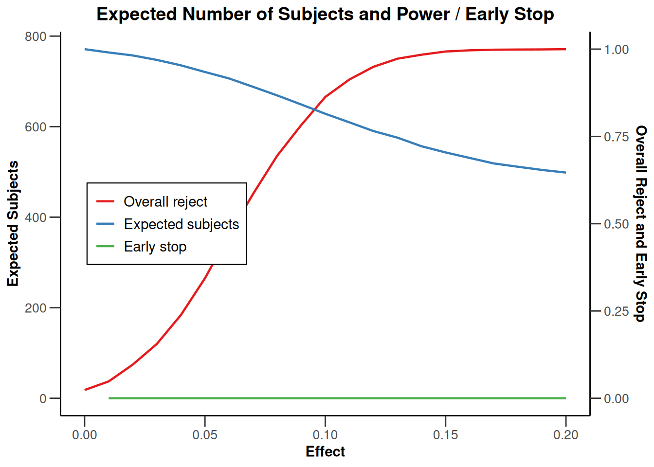
# Simulate designs again over a range of parameters and plot thempi1Seq <-seq(0.2, 0.4, by =0.01)simCpowerLong <-getSimulationRates(designIN,pi1 = pi1Seq, pi2 =0.2,plannedSubjects =c(2* n1, 2* Nmin),conditionalPower =0.9,minNumberOfSubjectsPerStage =c(2* n1, 2* (Nmin - n1)),maxNumberOfSubjectsPerStage =c(2* n1, 2* (Nmax - n1)),pi1H1 =0.3, pi2H1 =0.2,maxNumberOfIterations =10000,seed =12345)simCpowerLong |>plot(type =6)
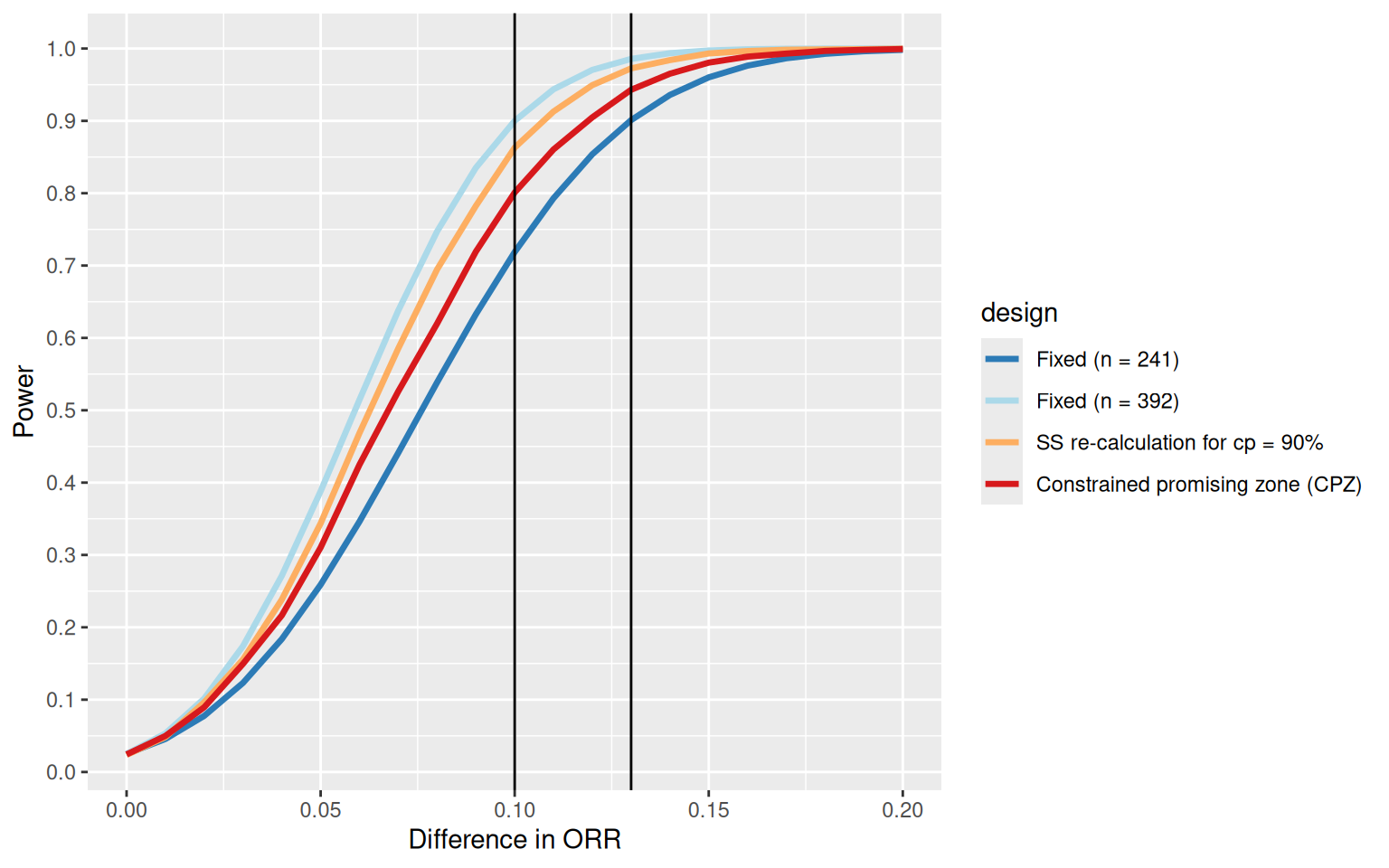
# Pool datasets from simulations (and fixed designs)simCpowerData <-with(as.list(simCpowerLong),data.frame(design ="SS re-calculation for cp = 90%",pi1 = pi1, pi2 = pi2, effect = effect, power = overallReject,expectedNumberOfSubjects1 = expectedNumberOfSubjects /2 ),stringsAsFactors = F)simCPZData <-with(as.list(simCPZLong),data.frame(design ="Constrained promising zone (CPZ)",pi1 = pi1, pi2 = pi2, effect = effect, power = overallReject,expectedNumberOfSubjects1 = expectedNumberOfSubjects /2 ),stringsAsFactors = F)simFixed241 <-with( simCPZData,data.frame(design ="Fixed (n = 241)",pi1 = pi1, pi2 = pi2, effect = effect,power =getPowerRates(pi1 = pi1, pi2 =0.2, maxNumberOfSubjects =2*241,alpha =0.025, sided =1 )$overallReject,expectedNumberOfSubjects1 =241, stringsAsFactors = F ))simFixed392 <-with( simCPZData,data.frame(design ="Fixed (n = 392)",pi1 = pi1, pi2 = pi2, effect = effect,power =getPowerRates(pi1 = pi1, pi2 =0.2, maxNumberOfSubjects =2*392,alpha =0.025, sided =1 )$overallReject,expectedNumberOfSubjects1 =392, stringsAsFactors = F ))simdata <-rbind(simCpowerData, simCPZData, simFixed241, simFixed392)simdata$design <-factor(simdata$design,levels =c("Fixed (n = 241)", "Fixed (n = 392)","SS re-calculation for cp = 90%", "Constrained promising zone (CPZ)" ))# Plot difference in ORR vs powerggplot(aes(effect, power, col = design), data = simdata) +geom_line(lwd =1.2) +scale_x_continuous(name ="Difference in ORR") +scale_y_continuous(breaks =seq(0, 1, by =0.1), name ="Power") +geom_vline(xintercept =c(0.1, 0.13), color ="black") +scale_color_manual(values =c("#2c7bb6", "#abd9e9", "#fdae61", "#d7191c"))
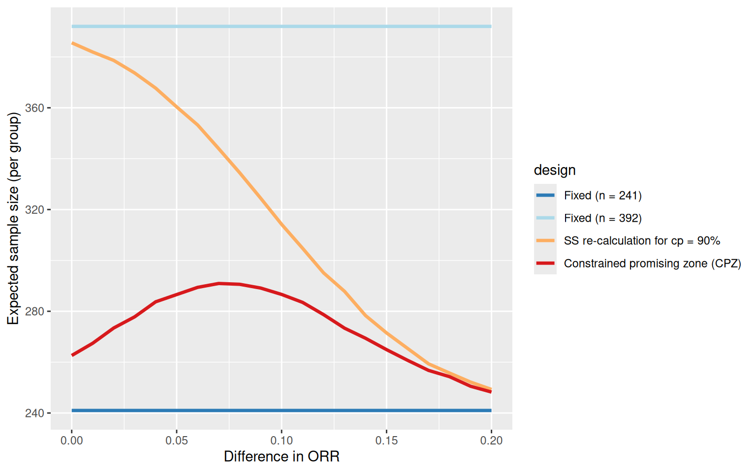
# Plot difference in ORR vs expected sample sizeggplot(aes(effect, expectedNumberOfSubjects1, col = design), data = simdata) +geom_line(lwd =1.2) +scale_x_continuous(name ="Difference in ORR") +scale_y_continuous(name ="Expected sample size (per group)") +scale_color_manual(values =c("#2c7bb6", "#abd9e9", "#fdae61", "#d7191c"))
Conclusions for the example
Targeting a fixed conditional power leads to the largest sample size increase if there is no treatment effect which is undesirable.
In contrast, the CPZ design increases sample size only if the interim Z-score is “promising”. The corresponding increase in the expected sample size is small if there is no treatment effect or if the treatment effect is large.
The CPZ design is a reasonable compromise between the two extreme fixed designs and has a power of approximately 80% for the smallest effect size of interest (\(\delta = 10\%\)).
Caveat: This is just a toy example and the design could be refined further (e.g., by exploring other SSR rules, changing the timing of the interim, or adding the possibility for a futility stop) and should also be compared to group sequential trial designs.
System: rpact 4.4.0.9305, R version 4.6.0 (2026-04-24), platform: x86_64-pc-linux-gnu
Wassmer G, Pahlke F (2026). rpact: Confirmatory Adaptive Clinical Trial Design and Analysis. R package version 4.4.0.9305. doi:10.32614/CRAN.package.rpact
Wassmer G, Brannath W (2025). Group Sequential and Confirmatory Adaptive Designs in Clinical Trials, 2nd edition. Springer, Cham, Switzerland. ISBN 978-3-031-89668-2. doi:10.1007/978-3-031-89669-9 https://doi.org/10.1007/978-3-031-89669-9.