packageVersion("rpact")[1] '5.0.0'In this vignette, we plan a hypothetical trial with two active doses and a common control. We first consider a single analysis, so that we can concentrate on specifying and interpreting the survival assumptions. We then extend the example to a two-stage design and compare continuing with all treatment arms with selecting the best arm at interim.
A treatment may improve survival only after patients have received it for some time. In this situation, a single hazard ratio does not describe the complete treatment effect. A piecewise exponential model allows the hazards in the control and treatment groups, and hence their ratios, to change at specified times. Via the function getPiecewiseSurvivalTimeMultiArm(), we can specify the hazards and then pass them directly to getSimulationMultiArmSurvival() to simulate patient accrual, event times, drop-out, and the analyses.
These features require rpact 5.0.0. Theversion used for the calculations below is:
packageVersion("rpact")[1] '5.0.0'We consider time to disease progression, measured in months. Lower hazards are favourable. Patients are initially allocated equally to low dose, high dose, and control. The study assumptions are illustrative; they do not represent estimates from a particular clinical trial.
| Assumption | Value |
|---|---|
| Active treatment arms | Low dose and high dose |
| Control survival | Exponential, with a median of 25 months |
| Treatment effect during the first six months | No difference from control |
| Treatment effect from month six onwards | HR 0.86 for low dose; HR 0.72 for high dose |
| Initial allocation | 1:1:1 across the three arms |
| Recruitment | 10 patients per month in months 0–12, 20 in months 12–24, and 40 in months 24–36 |
| Drop-out probability within 12 months | 1% for low dose and control; 2% for high dose |
| Analysis | One analysis after 460 events across the three arms (starting point for simulations) |
| Type I error | One-sided level 0.025 |
| Test | Dunnett intersection tests in the closed testing procedure |
Note that the event budget is merely a starting point to investigate further by simulation.
The interval starts refer to time since each patient’s study entry, not calendar time since the first patient was recruited. With starts at 0 and 6 months, the intervals are \([0,6)\) and \([6,\infty)\). (Note that the last interval is open-ended, so we do not need to add Inf to the vector.)
For exponential survival with median \(m\), the hazard is \(\lambda = \log(2)/m\). We use getLambdaByMedian() to obtain the control hazard and specify one value per interval, even though it is constant in this first example.
intervalStarts <- c(0, 6)
lambdaControl <- rep(getLambdaByMedian(25), 2)

hazardRatio <- rbind(
    lowDose = c(1, 0.72),
    highDose = c(1, 0.625)
)

piecewiseLambda <- getPiecewiseSurvivalTimeMultiArm(
    piecewiseSurvivalTime = intervalStarts,
    lambdaControl = lambdaControl,
    hazardRatio = hazardRatio
)

piecewiseLambda
Piecewise exponential multi-arm survival time
Control hazards (common to all comparisons)
| Interval | Control |
|---|---|
| 0 - <6 | 0.0277 |
| >=6 | 0.0277 |
Details
User defined parameters
Hazard ratios - Situation 1
| Interval | lowDose | highDose |
|---|---|---|
| 0 - <6 | 1.000 | 1.000 |
| >=6 | 0.720 | 0.625 |
Generated parameters
The hazard-ratio matrix has one row per active treatment arm and one column per interval, containing the values \(\text{HR}_{g,j}\) for each treatment arm \(g\) and interval \(j\). lambdaControl specifies the common control hazards \(\lambda_{C,j}\) for each interval \(j\). The treatment hazards are then calculated as \(\lambda_{g,j} = \text{HR}_{g,j}\lambda_{C,j}\).
The following table shows the resulting hazards. as.data.frame() provides one row for every treatment arm, interval, and simulation situation.
hazardTable <- as.data.frame(piecewiseLambda)
knitr::kable(
    hazardTable[c("group", "interval", "lambdaControl", "hazardRatio", "lambdaActive")],
    digits = 4,
    col.names = c("Treatment arm", "Interval", "Control hazard", "Hazard ratio", "Treatment hazard")
)| Treatment arm | Interval | Control hazard | Hazard ratio | Treatment hazard |
|---|---|---|---|---|
| lowDose | 0 - <6 | 0.0277 | 1.000 | 0.0277 |
| highDose | 0 - <6 | 0.0277 | 1.000 | 0.0277 |
| lowDose | >=6 | 0.0277 | 0.720 | 0.0200 |
| highDose | >=6 | 0.0277 | 0.625 | 0.0173 |
Control hazards are specified per month because all times in the example are in months. Hazards and hazard ratios must be finite and strictly positive. The control vector and every matrix must have one entry or column per interval; the function does not recycle values.
An alternative is to specify the exponential median associated with each interval’s hazard. Within the same interval, \(\text{HR} = \lambda_T/\lambda_C = m_C/m_T\). Consequently, a lower hazard ratio corresponds to a larger treatment median.
For example, a constant treatment HR of 0.72 against an exponential control median of 25 months corresponds to a treatment median of \(25/0.72 = 34.72\) months. A treatment median of 40 months against a control median of 25 months would instead correspond to HR \(25/40 = 0.625\), so smaller than the previous 0.72.
We now enter the same delayed-effect assumptions using medians:
medianControl <- c(25, 25)
medianTreatments <- rbind(
    lowDose = c(25, 34.72),
    highDose = c(25, 40)
)

piecewiseMedian <- getPiecewiseSurvivalTimeMultiArm(
    piecewiseSurvivalTime = intervalStarts,
    medianControl = medianControl,
    medianTreatments = medianTreatments
)

piecewiseMedian
Piecewise exponential multi-arm survival time
Control hazards (common to all comparisons)
| Interval | Control |
|---|---|
| 0 - <6 | 0.0277 |
| >=6 | 0.0277 |
Details
User defined parameters
Treatment medians - Situation 1 (exponential per interval)
| Interval | lowDose | highDose |
|---|---|---|
| 0 - <6 | 25.000 | 25.000 |
| >=6 | 34.720 | 40.000 |
Generated parameters
Hazard ratios - Situation 1
| Interval | lowDose | highDose |
|---|---|---|
| 0 - <6 | 1.000 | 1.000 |
| >=6 | 0.720 | 0.625 |
The function converts the medians with getLambdaByMedian(), using the exponential distribution with the default kappa = 1 argument. The original median inputs remain available on the object; the calculated hazards and hazard ratios are marked as derived parameters. The data-frame representations confirm that the two input forms describe the same survival distributions, up to numerical rounding:
all.equal(
    as.data.frame(piecewiseLambda),
    as.data.frame(piecewiseMedian),
    tolerance = 1e-4
)
[1] TRUEThe choices for control and treatment can also be made independently:
# Control medians together with treatment hazard ratios
piecewiseMixed1 <- getPiecewiseSurvivalTimeMultiArm(
    piecewiseSurvivalTime = intervalStarts,
    medianControl = medianControl,
    hazardRatio = hazardRatio
)

# Control hazards together with treatment medians
piecewiseMixed2 <- getPiecewiseSurvivalTimeMultiArm(
    piecewiseSurvivalTime = intervalStarts,
    lambdaControl = lambdaControl,
    medianTreatments = medianTreatments
)
Specify exactly one of lambdaControl and medianControl, and exactly one of hazardRatio and medianTreatments. Median inputs must be finite and positive and follow the same dimension and naming rules as the corresponding hazard inputs.
The median supplied for an interval describes the exponential distribution that would apply if that interval’s hazard continued indefinitely. It is not the actual median of the complete piecewise survival distribution.
For high dose, the entered values are 25 months for the first interval and 40 months for the second. Patients have already experienced six months of the control hazard before the lower hazard starts. The actual median from study entry is therefore different. We can calculate it from the complete distribution using getPiecewiseExponentialQuantile():
hazardsByArm <- rbind(
    lowDose = piecewiseLambda$getActiveHazards()[1, , 1],
    highDose = piecewiseLambda$getActiveHazards()[2, , 1],
    Control = lambdaControl
)

overallMedians <- vapply(seq_len(nrow(hazardsByArm)), function(arm) {
    return(getPiecewiseExponentialQuantile(
        quantile = 0.5,
        piecewiseSurvivalTime = intervalStarts,
        piecewiseLambda = hazardsByArm[arm, ]
    ))
}, numeric(1))

knitr::kable(
    data.frame(Arm = rownames(hazardsByArm), OverallMedian = overallMedians),
    digits = 2,
    col.names = c("Arm", "Actual median from study entry (months)")
)| Arm | Actual median from study entry (months) |
|---|---|
| lowDose | 32.39 |
| highDose | 36.40 |
| Control | 25.00 |
For high dose, the actual median is approximately 36.4 months, rather than 40 months. In this particular example, it can also be obtained as \(6 + (25 - 6)/0.625\). That expression uses the fact that the 50% survival point occurs after the change in hazard.
The distributions can be inspected before running a simulation. getPiecewiseExponentialDistribution() returns cumulative event probabilities, so we subtract them from one to obtain survival probabilities.
timeGrid <- seq(0, 60, by = 0.25)
survivalCurves <- data.frame(
    time = rep(timeGrid, times = nrow(hazardsByArm)),
    arm = rep(rownames(hazardsByArm), each = length(timeGrid))
) |>
    dplyr::group_by(arm) |>
    dplyr::mutate(survival = 1 - getPiecewiseExponentialDistribution(
        time = time,
        piecewiseSurvivalTime = intervalStarts,
        piecewiseLambda = hazardsByArm[match(dplyr::first(arm), rownames(hazardsByArm)), ]
    )) |>
    dplyr::ungroup()
survivalCurves$arm <- factor(survivalCurves$arm, levels = rownames(hazardsByArm))

ggplot(survivalCurves, aes(time, survival, colour = arm)) +
    geom_line(linewidth = 0.9) +
    geom_vline(xintercept = 6, linetype = "dashed", colour = "grey50") +
    scale_colour_manual(
        values = c(lowDose = "#0072B2", highDose = "#009E73", Control = "#666666"),
        labels = c("Low dose", "High dose", "Control")
    ) +
    labs(x = "Months since study entry", y = "Probability of no progression", colour = "Arm") +
    theme_minimal()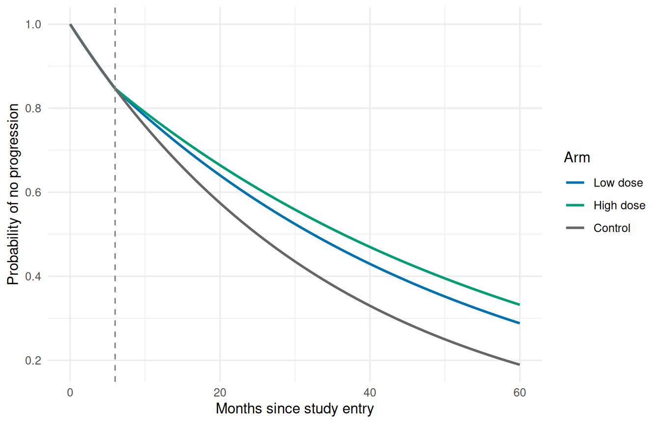
Other control-hazard patterns can be entered by changing the two control values; they need not be identical. Such interval medians would then no longer, in general, equal the actual overall control median either.
We first define the recruitment and drop-out assumptions. The recruitment scheme allows a maximum of 840 patients:
accrualTime <- c(0, 12, 24, 36)
accrualIntensity <- c(10, 20, 40)
maxNumberOfSubjects <- sum(diff(accrualTime) * accrualIntensity)
maxNumberOfSubjects
[1] 840We explicitly select the C++ patient-wise engine with simulationType = "patientWise". Note that a piecewise hazards specification could not be used with the test-statistic based simulations. allocationRatioPlanned = 1 gives equal allocation to each active arm and control at the start. Drop-out is independent and exponentially distributed, with the specified probabilities referring to dropoutTime = 12 months. In the output we also see the resulting drop-out proportions at the analysis time of about 60 months in each of the arms.
maxNumberOfIterations <- 5000
designFixed <- getDesignFixed(alpha = 0.025, sided = 1)

simulationFixed <- getSimulationMultiArmSurvival(
    design = designFixed,
    piecewiseSurvivalTime = piecewiseLambda,
    simulationType = "patientWise",
    directionUpper = FALSE,
    intersectionTest = "Dunnett",
    typeOfSelection = "all",
    plannedEvents = 460,
    allocationRatioPlanned = 1,
    accrualTime = accrualTime,
    accrualIntensity = accrualIntensity,
    accrualIntensityType = "absolute",
    maxNumberOfSubjects = maxNumberOfSubjects,
    dropoutRate1 = c(0.01, 0.02),
    dropoutRate2 = 0.01,
    dropoutTime = 12,
    maxNumberOfIterations = maxNumberOfIterations,
    seed = 1234
)

summary(simulationFixed)
Simulation of a survival endpoint (multi-arm design)
Fixed sample analysis, one-sided significance level 2.5%. The results were obtained using patient-level simulation for a multi-arm logrank test (2 treatments vs. control), H0: hazard ratio(i) = 1, power directed towards smaller values, H1: piecewise exponential survival distribution with interval start times = c(0, 6) (last interval open-ended), common control hazards = c(0.0277, 0.0277), hazard ratios for Situation 1 (in interval order): lowDose = c(1, 0.72); highDose = c(1, 0.625), planned events = 460, number of subjects = 840, accrual time = c(12, 24, 36), accrual intensity = c(10, 20, 40), dropout rate(1) = c(0.01, 0.02), dropout rate(2) = 0.01, dropout time = 12, effect shape = user defined, intersection test = Dunnett, success criterion: all, simulation runs = 5000, seed = 1234.
| Stage | Fixed |
|---|---|
| Stage level (one-sided) | 0.0250 |
| Efficacy boundary (z-value scale) | 1.960 |
| Reject at least one | 0.8254 |
| Rejected arms | |
| Treatment arm 1 vs. control | 0.5452 |
| Treatment arm 2 vs. control | 0.7984 |
| Number of subjects | 840.0 |
| Cumulative number of events | |
| Treatment arm 1 vs. control | 323.5 |
| Treatment arm 2 vs. control | 311.0 |
| Analysis time | 60.31 |
| Expected study duration | 60.31 |
| Observed drop-out proportion | |
| Treatment arm 1 | 0.0203 |
| Treatment arm 2 | 0.0421 |
| Control | 0.0187 |
The estimated probability of rejecting at least one treatment hypothesis in this delayed-effect scenario is 82.5%. This is power to demonstrate a benefit for at least one dose, not the probability of demonstrating both doses or the power of each individual comparison. The two treatment arms have different effects, so individual rejection probabilities differ and we see them separately reported in the table above. Their sum need not equal the probability of rejecting at least one hypothesis because both doses can be significant in the same trial. We can look at these in more detail now by extracting them from the rejectedArmsPerStage element of the result:
summarizeDoseRejections <- function(result, strategy, situations) {
    doseProbabilities <- apply(result$rejectedArmsPerStage, c(2, 3), sum)
    probability <- as.vector(doseProbabilities)
    return(data.frame(
        Strategy = strategy,
        Situation = rep(situations, times = 2),
        Dose = rep(c("Low dose", "High dose"), each = length(situations)),
        RejectionProbability = probability,
        MonteCarloSE = sqrt(probability * (1 - probability) / maxNumberOfIterations)
    ))
}

fixedDoseRejections <- summarizeDoseRejections(simulationFixed, "Single stage", "delayed")
knitr::kable(
    fixedDoseRejections[c("Dose", "RejectionProbability", "MonteCarloSE")],
    digits = c(0, 3, 4),
    col.names = c("Dose", "Rejection probability", "Monte Carlo SE")
)| Dose | Rejection probability | Monte Carlo SE |
|---|---|---|
| Low dose | 0.545 | 0.0070 |
| High dose | 0.798 | 0.0057 |
The Monte Carlo standard error used above is \(\sqrt{\widehat p(1-\widehat p)/N}\), where \(N\) is the number of simulated trials in that situation.
rejectedArmsPerStage has dimensions stages x situations x active arms. Summing over stages gives the probability of rejecting each dose by the end of the trial. In this single-stage example, the stage dimension has length one.
The estimated study duration is 60.3 months. Recruitment stops at the patient limit, but observation continues to obtain the event target. Check eventsNotAchieved whenever recruitment or drop-out could prevent enough events from being observed:
simulationFixed$eventsNotAchieved [,1]
[1,] 0Here it is zero, indicating that the event target was achieved in all simulated trials.
Now we add an interim analysis and allow for treatment-arm selection based on the observed data.
We want to evaluate four different situations of the hazard ratios vs. control:
| Situation | First six months | From month six onwards |
|---|---|---|
immediate |
HR 0.86 for low dose; HR 0.72 for high dose | Same effects continue |
delayed |
HR 1 for both doses | HR 0.86 for low dose; HR 0.72 for high dose |
globalNull |
HR 1 for both doses | HR 1 for both doses |
partialNull |
HR 1 for both doses | HR 1 for low dose; HR 0.72 for high dose |
The globalNull situation provides a simulation check of the probability of rejecting at least one hypothesis when neither dose is effective. In the partialNull situation, low dose remains ineffective while high dose has a delayed benefit.
We specify these situations with a named list of arm-by-interval matrices. Matrix rows and their names must agree across situations, including their order. Let’s do that:
hazardRatioSituations <- list(
    immediate = rbind(
        lowDose = c(0.86, 0.86),
        highDose = c(0.72, 0.72)
    ),
    delayed = rbind(
        lowDose = c(1, 0.86),
        highDose = c(1, 0.72)
    ),
    globalNull = rbind(
        lowDose = c(1, 1),
        highDose = c(1, 1)
    ),
    partialNull = rbind(
        lowDose = c(1, 1),
        highDose = c(1, 0.72)
    )
)

piecewiseSituations <- getPiecewiseSurvivalTimeMultiArm(
    piecewiseSurvivalTime = intervalStarts,
    lambdaControl = lambdaControl,
    hazardRatio = hazardRatioSituations
)

piecewiseSituations
Piecewise exponential multi-arm survival time
Control hazards (common to all comparisons)
| Interval | Control |
|---|---|
| 0 - <6 | 0.0277 |
| >=6 | 0.0277 |
Details
User defined parameters
Hazard ratios - immediate
| Interval | lowDose | highDose |
|---|---|---|
| 0 - <6 | 0.860 | 0.720 |
| >=6 | 0.860 | 0.720 |
Hazard ratios - delayed
| Interval | lowDose | highDose |
|---|---|---|
| 0 - <6 | 1.000 | 1.000 |
| >=6 | 0.860 | 0.720 |
Hazard ratios - globalNull
| Interval | lowDose | highDose |
|---|---|---|
| 0 - <6 | 1.000 | 1.000 |
| >=6 | 1.000 | 1.000 |
Hazard ratios - partialNull
| Interval | lowDose | highDose |
|---|---|---|
| 0 - <6 | 1.000 | 1.000 |
| >=6 | 1.000 | 0.720 |
Generated parameters
Note that internally an array is used to store the hazard ratios, with dimensions corresponding to active arm, interval, and situation. The helper getPiecewiseHazardRatioArray() can create the same array explicitly if needed.
Both a named list and the equivalent array can also be used for the specification of median survival times. For example, the following median specification reproduces all four situations:
medianTreatmentSituations <- lapply(hazardRatioSituations, function(ratios) {
    return(25 / ratios)
})

piecewiseSituationMedians <- getPiecewiseSurvivalTimeMultiArm(
    piecewiseSurvivalTime = intervalStarts,
    medianControl = medianControl,
    medianTreatments = medianTreatmentSituations
)

all.equal(
    as.data.frame(piecewiseSituations),
    as.data.frame(piecewiseSituationMedians),
    tolerance = 1e-12
)
[1] TRUEFinally, note that all situations share the control-hazard vector. To investigate different control distributions or recruitment schemes, you need to run separate specifications and simulations.
We use an inverse-normal combination design with one interim analysis. There is no early efficacy stop. The interim futility boundary is zero (on the \(z\)-scale), corresponding to a hazard ratio of 1, and the planned cumulative event budgets are 230 and 460.
designTwoStage <- getDesignInverseNormal(
    kMax = 2,
    typeOfDesign = "noEarlyEfficacy",
    alpha = 0.025,
    futilityBounds = 0
)
We compare two strategies using this same design:
"all": retain all active arms if the trial continues, subject to the futility rule."best": select the arm with the most favourable observed treatment effect if the trial continues. With directionUpper = FALSE, a lower estimated HR is favourable.To keep the comparison reproducible, we first collect the common simulation arguments in a list and afterwards use do.call to run the simulations with the two different selection rules:
simulationArguments <- list(
    design = designTwoStage,
    piecewiseSurvivalTime = piecewiseSituations,
    simulationType = "patientWise",
    directionUpper = FALSE,
    intersectionTest = "Dunnett",
    effectMeasure = "effectEstimate",
    plannedEvents = c(230, 460),
    allocationRatioPlanned = 1,
    accrualTime = accrualTime,
    accrualIntensity = accrualIntensity,
    accrualIntensityType = "absolute",
    maxNumberOfSubjects = maxNumberOfSubjects,
    dropoutRate1 = c(0.01, 0.02),
    dropoutRate2 = 0.01,
    dropoutTime = 12,
    maxNumberOfIterations = maxNumberOfIterations,
    maxNumberOfRawDatasetsPerStage = 1,
    seed = 1234
)

simulationAll <- do.call(
    getSimulationMultiArmSurvival,
    c(simulationArguments, list(typeOfSelection = "all"))
)
simulationBest <- do.call(
    getSimulationMultiArmSurvival,
    c(simulationArguments, list(typeOfSelection = "best"))
)plannedEvents = c(230, 460) specifies 230 events up to interim and 230 additional events for the next stage. Therefore in total, the trial plans for 460 events. Once an arm has been dropped, its events observed after exclusion no longer contribute to the next analysis. Events previously observed in that arm remain part of the event budget already spent.
For example, suppose the retained treatment arm and the control arm together have 153 events at interim. The final analysis then requires 153 + 230 = 383 events in that retained pair, rather than 460 events in the pair. The 230 additional events can include events observed after interim in patients who had already entered the retained arms, as well as events in newly recruited patients.
The following table reports the rejection probability, its Monte Carlo standard error, the expected number of patients, and the expected study duration. In immediate and delayed, the rejection probability is the power to demonstrate at least one effective dose. In globalNull, it estimates the family-wise Type I error probability. In partialNull, it includes both correct rejections of high dose and erroneous rejections of low dose, so it must not be interpreted as either pure efficacy power or family-wise Type I error.
situationNames <- dimnames(piecewiseSituations$hazardRatio)$situation
summarizeSimulation <- function(result, strategy) {
    probability <- result$rejectAtLeastOne
    return(data.frame(
        Strategy = strategy,
        Situation = situationNames,
        RejectionProbability = probability,
        MonteCarloSE = sqrt(probability * (1 - probability) / maxNumberOfIterations),
        ExpectedPatients = result$expectedNumberOfSubjects,
        ExpectedDuration = result$studyDuration
    ))
}

comparison <- rbind(
    summarizeSimulation(simulationAll, "All arms"),
    summarizeSimulation(simulationBest, "Best arm")
)
knitr::kable(
    comparison,
    digits = c(0, 0, 3, 4, 1, 1),
    col.names = c("Strategy", "Situation", "Reject at least one",
        "Monte Carlo SE", "Expected patients", "Expected duration (months)")
)| Strategy | Situation | Reject at least one | Monte Carlo SE | Expected patients | Expected duration (months) |
|---|---|---|---|---|---|
| All arms | immediate | 0.721 | 0.0063 | 840.0 | 57.8 |
| All arms | delayed | 0.424 | 0.0070 | 839.6 | 53.5 |
| All arms | globalNull | 0.023 | 0.0021 | 833.5 | 44.7 |
| All arms | partialNull | 0.360 | 0.0068 | 839.0 | 51.4 |
| Best arm | immediate | 0.814 | 0.0055 | 840.0 | 73.8 |
| Best arm | delayed | 0.498 | 0.0071 | 839.6 | 66.0 |
| Best arm | globalNull | 0.028 | 0.0023 | 833.7 | 51.3 |
| Best arm | partialNull | 0.481 | 0.0071 | 839.0 | 63.9 |
The per-dose probabilities separate these conclusions:
doseRejections <- rbind(
    summarizeDoseRejections(simulationAll, "All arms", situationNames),
    summarizeDoseRejections(simulationBest, "Best arm", situationNames)
)
knitr::kable(
    doseRejections,
    digits = c(0, 0, 0, 3, 4),
    col.names = c("Strategy", "Situation", "Dose", "Rejection probability", "Monte Carlo SE")
)| Strategy | Situation | Dose | Rejection probability | Monte Carlo SE |
|---|---|---|---|---|
| All arms | immediate | Low dose | 0.266 | 0.0062 |
| All arms | delayed | Low dose | 0.145 | 0.0050 |
| All arms | globalNull | Low dose | 0.014 | 0.0017 |
| All arms | partialNull | Low dose | 0.020 | 0.0020 |
| All arms | immediate | High dose | 0.714 | 0.0064 |
| All arms | delayed | High dose | 0.409 | 0.0070 |
| All arms | globalNull | High dose | 0.013 | 0.0016 |
| All arms | partialNull | High dose | 0.359 | 0.0068 |
| Best arm | immediate | Low dose | 0.069 | 0.0036 |
| Best arm | delayed | Low dose | 0.065 | 0.0035 |
| Best arm | globalNull | Low dose | 0.013 | 0.0016 |
| Best arm | partialNull | Low dose | 0.007 | 0.0012 |
| Best arm | immediate | High dose | 0.745 | 0.0062 |
| Best arm | delayed | High dose | 0.434 | 0.0070 |
| Best arm | globalNull | High dose | 0.015 | 0.0017 |
| Best arm | partialNull | High dose | 0.474 | 0.0071 |
For partialNull, the high-dose rejection probability is power for the effective dose. The low-dose rejection probability is the family-wise Type I error probability because low dose is the only true null hypothesis in this situation.
Selecting one arm concentrates subsequent events on a single treatment-control comparison. Any improvement in rejection probability must be assessed together with the longer time that may be needed to observe those events. For the best-arm strategy, the estimated rejection probabilities are 81.4% with immediate effects and 49.8% with delayed effects. If we wanted to have a 90% power we would further need to increase the number of events accordingly.
Under delayed effects, retaining the best arm changes the rejection probability from 42.4% to 49.8%, while expected study duration changes from 53.5 to 66 months. Expected recruitment is the same (839.6 patients), respectively. Thus, the gain in rejection probability comes with longer follow-up.
For each strategy, we report the probability of rejecting at least one true null hypothesis under the global and partial null. An exact binomial confidence interval describes the uncertainty from the finite simulation:
summarizeTypeIError <- function(result, strategy) {
    globalNullIndex <- match("globalNull", situationNames)
    partialNullIndex <- match("partialNull", situationNames)
    probability <- c(
        result$rejectAtLeastOne[globalNullIndex],
        sum(result$rejectedArmsPerStage[, partialNullIndex, 1])
    )
    intervals <- vapply(probability, function(p) {
        return(stats::binom.test(
            x = round(p * maxNumberOfIterations),
            n = maxNumberOfIterations,
            conf.level = 0.95
        )$conf.int)
    }, numeric(2))
    return(data.frame(
        Strategy = strategy,
        Situation = c("globalNull", "partialNull"),
        TypeIError = probability,
        MonteCarloSE = sqrt(probability * (1 - probability) / maxNumberOfIterations),
        Lower95 = intervals[1, ],
        Upper95 = intervals[2, ]
    ))
}

typeIErrorPrecision <- rbind(
    summarizeTypeIError(simulationAll, "All arms"),
    summarizeTypeIError(simulationBest, "Best arm")
)
knitr::kable(
    typeIErrorPrecision,
    digits = c(0, 0, 4, 4, 4, 4),
    col.names = c("Strategy", "Situation", "Type I error", "Monte Carlo SE", "Lower 95%", "Upper 95%")
)| Strategy | Situation | Type I error | Monte Carlo SE | Lower 95% | Upper 95% |
|---|---|---|---|---|---|
| All arms | globalNull | 0.0226 | 0.0021 | 0.0187 | 0.0271 |
| All arms | partialNull | 0.0200 | 0.0020 | 0.0163 | 0.0243 |
| Best arm | globalNull | 0.0278 | 0.0023 | 0.0234 | 0.0327 |
| Best arm | partialNull | 0.0070 | 0.0012 | 0.0049 | 0.0097 |
More iterations estimate the actual rejection probability more precisely. At a probability near 0.025, about 94,000 iterations are needed for a rough 95% margin of 0.1 percentage points, using \(N \approx 1.96^2 \times 0.025 \times 0.975 / 0.001^2\). With this we can choose the number of simulations based on the precision target before the final evaluation run.
The inverse-normal combination design with closed testing accommodates treatment selection and strong control of the family-wise error rate, subject to the validity of its stagewise tests and their assumptions. Here the survival tests use large-sample approximations; the nominal level is not a guarantee of exact finite-sample family-wise error control below 0.025. Interim futility can also make the procedure conservative. The global null and this single partial-null example are illustrative scenarios, but they do not establish strong control over all configurations.
We can display the situation-specific rejection probabilities directly with the rpact plot method:
plot(simulationBest, type = 1)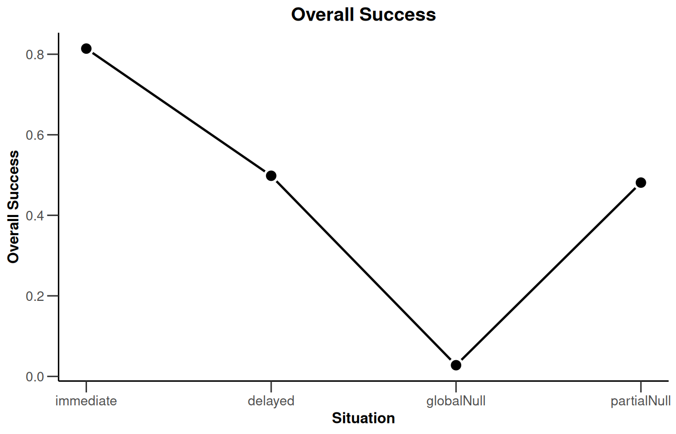
The x-axis identifies the situations, rather than using the initial HR as a numerical coordinate. This is important because the delayed and null situations have identical initial HRs but different later effects.
Selection probabilities help distinguish failure to continue from selecting the less effective dose. The probabilities below are unconditional: each is the probability that a simulated trial reaches stage 2 with that arm selected. For "best", their sum is the probability of reaching stage 2, i.e. not be stopped for futility.
selectionTable <- data.frame(
    Situation = situationNames,
    LowDoseRetained = simulationBest$selectedArms[2, , 1],
    HighDoseRetained = simulationBest$selectedArms[2, , 2],
    ReachesStage2 = simulationBest$iterations[2, ] / maxNumberOfIterations
)
knitr::kable(
    selectionTable,
    digits = c(0, 3, 3, 3),
    col.names = c("Situation", "Low dose retained", "High dose retained", "Reaches stage 2")
)| Situation | Low dose retained | High dose retained | Reaches stage 2 |
|---|---|---|---|
| immediate | 0.135 | 0.832 | 0.967 |
| delayed | 0.226 | 0.580 | 0.806 |
| globalNull | 0.259 | 0.242 | 0.501 |
| partialNull | 0.116 | 0.650 | 0.766 |
Next, let’s compare the interim timing with the planned end of recruitment at month 36. getData() contains one record per active arm and analysis. We select the first-stage record for arm 1 so that every simulated trial is counted once:
analysisData <- getData(simulationBest)
interimAfterRecruitment <- analysisData |>
    dplyr::filter(stageNumber == 1, activeArm == 1) |>
    dplyr::group_by(scenario) |>
    dplyr::summarise(
        interimAfterRecruitment = mean(analysisTime >= max(accrualTime)),
        .groups = "drop"
    ) |>
    dplyr::arrange(scenario) |>
    dplyr::pull(interimAfterRecruitment)

timingTable <- data.frame(
    Situation = situationNames,
    MeanInterimTime = simulationBest$analysisTime[1, ],
    InterimAfterRecruitment = interimAfterRecruitment
)
knitr::kable(
    timingTable,
    digits = c(0, 1, 3),
    col.names = c("Situation", "Mean interim time (months)", "Probability of interim at or after month 36")
)| Situation | Mean interim time (months) | Probability of interim at or after month 36 |
|---|---|---|
| immediate | 37.8 | 0.986 |
| delayed | 36.9 | 0.870 |
| globalNull | 36.0 | 0.467 |
| partialNull | 36.6 | 0.761 |
Under this recruitment scheme, the interim analysis often takes place after recruitment is complete, so arm selection offers little opportunity to reduce the number of recruited patients. If reducing recruitment is an important objective, its timing relative to the interim event target would need to be reconsidered.
Event-target failures also need to be checked for both strategies. The entries below are proportions, reported separately for each stage and situation:
simulationAll$eventsNotAchieved [,1] [,2] [,3] [,4]
[1,] 0 0 0 0
[2,] 0 0 0 0simulationBest$eventsNotAchieved [,1] [,2] [,3] [,4]
[1,] 0 0 0 0
[2,] 0 0 0 0For diagnostic purposes and to keep the data small, we retained above at most one raw dataset per situation and stopping stage.
rawData <- getRawData(simulationBest)
head(rawData[c("scenario", "iterationNumber", "treatmentGroup", "survivalTime", "timeUnderObservation")])
scenario iterationNumber treatmentGroup survivalTime timeUnderObservation
1 1 1 1 16.348774 16.348774
2 1 1 2 225.126336 69.854110
3 1 1 3 7.028003 7.028003
4 1 1 1 3.772382 3.772382
5 1 1 2 47.980438 47.980438
6 1 1 3 63.567334 63.567334Here, treatmentGroup 1 denotes low dose, 2 denotes high dose, and the last group 3 denotes control. Control is last in the three-arm trial, just as it is arm 2 in a two-arm trial. The scenario values follow the order immediate, delayed, globalNull, partialNull. A generated survivalTime can exceed timeUnderObservation, indicating a censored observation.
For an actual planning exercise, the next steps would include varying the delay and effect sizes, checking whether more events are needed, and examining less aggressive futility rules or a different interim timing. The 460-event budget is an illustrative candidate; simulation results under delayed effects must guide its assessment. Increase maxNumberOfIterations for the final evaluation and report Monte Carlo uncertainty, especially when assessing rejection probabilities near the nominal Type I error level.
Further examples are provided in Planning a Survival Trial with rpact and Simulation-Based Design of Group Sequential Trials with a Survival Endpoint.