library(rpact)
packageVersion("rpact") # version should be version 3.0.1 or laterSimulating Multi-Arm Designs with a Continuous Endpoint using rpact
Planning
Means
Power simulation
Multi-arm
This document provides examples for simulating multi-arm multi-stage (MAMS) designs for testing means with rpact.
Introduction
This document provides examples for simulating multi-arm multi-stage (MAMS) designs for testing means in many-to-one comparisons. For designs with multiple arms, rpact enables the simulation of designs that use the closed combination testing principle. For a description of the methodology please refer to Part III of the book “Group Sequential and Confirmatory Adaptive Designs in Clinical Trials” by Gernot Wassmer & Werner Brannath. Essentially, we show in this vignette how to reproduce part of the simulation results provided in the paper “On Sample Size Determination in Multi-Arm Confirmatory Adaptive Designs” by Gernot Wassmer (Journal of Biopharmaceutical Statistics, 2011).
First, load the rpact package
[1] '4.0.0'Sample size calculation for the adaptive multi-arm situation
rpact enables the assessment of sample sizes in multiple arms including selection of treatment arms. We will first consider the simple case of a two-stage design with O’Brien & Fleming boundaries assuming three active treatment arms which are tested against control. Let the three treatment arms be referring to three different and increasing doses, “low”, “medium”, and “high”, say. We assume that the highest dose will have response difference 10 as compared to control, and that there will be a linear dose-response relationship. The standard deviation is assumed to be \(\sigma = 15\). At interim, the treatment arm with the highest observed response as compared to placebo is selected for testing at the second stage.
One way to adjust for the multiple comparison situation is to use the Bonferroni correction for testing the intersection tests in the closed system of hypotheses. It will show that using \(\alpha/3\) instead of \(\alpha\) for the sample size calculation for the highest dose in the two-arm fixed sample size case can serve as a reasonable first guess for the sample size for the multi-arm case. That is, for \(\alpha = 0.025\) and power \(1 - \beta = 90\%\) we calculate the sample size using the commands
nsFixed <- getSampleSizeMeans(alpha = 0.025 / 3, beta = 0.1, alternative = 10, stDev = 15)
kable(summary(nsFixed))
Warning in is.na(parameterValues): is.na() auf Nicht-(Liste oder Vektor) des
Typs 'environment' angewendet| object | NA | NA | NA | NA | NA | NA | NA | NA | NA | NA | NA |
|---|---|---|---|---|---|---|---|---|---|---|---|
| 1 | 10 | FALSE | 0 | FALSE | 15 | 2 | 1 | 124.4932 | 62.24661 | 62.24661 | 6.526379 |
yielding 125 as the total number of subjects and hence n = 63 subjects per treatment arm in order to achieve the desired power. As a first guess for the multi-arm two-stage case we choose 30 per stage and treatment arm and use the following commands for evaluating the MAMS design. Note that plannedSubjects refers to the cumulative sample sizes over the stages per selected active arm:
designIN <- getDesignInverseNormal(kMax = 2, alpha = 0.025, typeOfDesign = "OF")
maxNumberOfIterations <- 1000
simBonfMAMS <- getSimulationMultiArmMeans(
    design = designIN,
    activeArms = 3,
    muMaxVector = c(10),
    stDev = 15,
    plannedSubjects = c(30, 60),
    intersectionTest = "Bonferroni",
    typeOfShape = "linear",
    typeOfSelection = "best",
    successCriterion = "all",
    maxNumberOfIterations = maxNumberOfIterations,
    seed = 1234
)
kable(summary(simBonfMAMS))
Warning in is.na(parameterValues): is.na() auf Nicht-(Liste oder Vektor) des
Typs 'environment' angewendet| object | NA | NA | NA | NA | NA | NA | NA | NA | NA | NA | NA | NA | NA | NA | NA | NA | NA | NA | NA | NA | NA | NA | NA | NA | NA | NA |
|---|---|---|---|---|---|---|---|---|---|---|---|---|---|---|---|---|---|---|---|---|---|---|---|---|---|---|
| 1 | 1000 | 1234 | 1 | 0.004 | 15 | 30 | 3 | 10 | linear | 10 | 1 | Bonferroni | best | effectEstimate | all | NA | NA | -Inf | 1000 | 0.885 | 0.004 | 0.01 | 0.006 | 3 | 179.4 | NA |
| 2 | 1000 | 1234 | 1 | 0.004 | 15 | 60 | 3 | 10 | linear | 10 | 1 | Bonferroni | best | effectEstimate | all | NA | NA | -Inf | 990 | 0.885 | NA | NA | 0.879 | 1 | 179.4 | 0.578451 |
We see that the power, which is the probability to reject at least one of the three corresponding hypotheses, is about 88% if a linear dose-response relationship is assumed. Note that there is a small probability to stop the trial for futility which is due to the use of the Bonferroni correction yielding adjusted \(p\)-values equal to 1 at interim (making a rejection at stage 2 impossible).
Using the Dunnett test for testing the intersection hypotheses increases the power to about 90% which is obtained by selecting intersectionTest = "Dunnett":
simDunnettMAMS <- getSimulationMultiArmMeans(
    design = designIN,
    activeArms = 3,
    typeOfShape = "linear",
    muMaxVector = c(10),
    stDev = 15,
    plannedSubjects = c(30, 60),
    intersectionTest = "Dunnett",
    typeOfSelection = "best",
    successCriterion = "all",
    maxNumberOfIterations = maxNumberOfIterations,
    seed = 1234
)
kable(summary(simDunnettMAMS))
Warning in is.na(parameterValues): is.na() auf Nicht-(Liste oder Vektor) des
Typs 'environment' angewendet| object | NA | NA | NA | NA | NA | NA | NA | NA | NA | NA | NA | NA | NA | NA | NA | NA | NA | NA | NA | NA | NA | NA | NA | NA | NA | NA |
|---|---|---|---|---|---|---|---|---|---|---|---|---|---|---|---|---|---|---|---|---|---|---|---|---|---|---|
| 1 | 1000 | 1234 | 1 | 0 | 15 | 30 | 3 | 10 | linear | 10 | 1 | Dunnett | best | effectEstimate | all | NA | NA | -Inf | 1000 | 0.899 | 0 | 0.006 | 0.006 | 3 | 179.64 | NA |
| 2 | 1000 | 1234 | 1 | 0 | 15 | 60 | 3 | 10 | linear | 10 | 1 | Dunnett | best | effectEstimate | all | NA | NA | -Inf | 994 | 0.899 | NA | NA | 0.893 | 1 | 179.64 | 0.5761233 |
Changing successCriterion = "all" to successCriterion = "atLeastOne" reduces the expected number of subjects considerably because the trial is stopped at interim in many more cases:
simDunnettMAMSatLeastOne <- getSimulationMultiArmMeans(
    design = designIN,
    activeArms = 3,
    typeOfShape = "linear",
    muMaxVector = c(10),
    stDev = 15,
    plannedSubjects = c(30, 60),
    intersectionTest = "Dunnett",
    typeOfSelection = "best",
    successCriterion = "atLeastOne",
    maxNumberOfIterations = maxNumberOfIterations,
    seed = 1234
)
kable(summary(simDunnettMAMSatLeastOne))
Warning in is.na(parameterValues): is.na() auf Nicht-(Liste oder Vektor) des
Typs 'environment' angewendet| object | NA | NA | NA | NA | NA | NA | NA | NA | NA | NA | NA | NA | NA | NA | NA | NA | NA | NA | NA | NA | NA | NA | NA | NA | NA | NA |
|---|---|---|---|---|---|---|---|---|---|---|---|---|---|---|---|---|---|---|---|---|---|---|---|---|---|---|
| 1 | 1000 | 1234 | 1 | 0 | 15 | 30 | 3 | 10 | linear | 10 | 1 | Dunnett | best | effectEstimate | atLeastOne | NA | NA | -Inf | 1000 | 0.899 | 0 | 0.342 | 0.342 | 3 | 159.48 | NA |
| 2 | 1000 | 1234 | 1 | 0 | 15 | 60 | 3 | 10 | linear | 10 | 1 | Dunnett | best | effectEstimate | atLeastOne | NA | NA | -Inf | 658 | 0.899 | NA | NA | 0.557 | 1 | 159.48 | 0.3988859 |
For this example, we might conclude that choosing 30 subjects per treatment arm and stage is a reasonable choice. If, however, the effect sizes are smaller for the low and medium dose, the power might decrease and the sample size therefore should be increased. For example, assuming effect sizes of only 1 and 2 in the low and medium dose group, respectively, the test characteristics can be obtained by using the typeOfShape = userDefined option. The effect sizes of interest are specified through effectMatrix (which needs to be a matrix because you can also generally consider more that one parameter configuration per simulation run):
simDunnettMAMS <- getSimulationMultiArmMeans(
    design = designIN,
    activeArms = 3,
    typeOfShape = "userDefined",
    effectMatrix = matrix(c(1, 2, 10), ncol = 3),
    stDev = 15,
    plannedSubjects = c(30, 60),
    intersectionTest = "Dunnett",
    typeOfSelection = "best",
    successCriterion = "atLeastOne",
    maxNumberOfIterations = maxNumberOfIterations,
    seed = 1234
)
kable(summary(simDunnettMAMS))
Warning in is.na(parameterValues): is.na() auf Nicht-(Liste oder Vektor) des
Typs 'environment' angewendet| object | NA | NA | NA | NA | NA | NA | NA | NA | NA | NA | NA | NA | NA | NA | NA | NA | NA | NA | NA | NA | NA | NA | NA | NA | NA | NA |
|---|---|---|---|---|---|---|---|---|---|---|---|---|---|---|---|---|---|---|---|---|---|---|---|---|---|---|
| 1 | 1000 | 1234 | 1 | 0 | 15 | 30 | 3 | 1 | userDefined | 10 | 1 | Dunnett | best | effectEstimate | atLeastOne | NA | NA | -Inf | 1000 | 0.897 | 0 | 0.306 | 0.306 | 3 | 161.64 | NA |
| 2 | 1000 | 1234 | 1 | 0 | 15 | 60 | 3 | 1 | userDefined | 10 | 1 | Dunnett | best | effectEstimate | atLeastOne | NA | NA | -Inf | 694 | 0.897 | NA | NA | 0.591 | 1 | 161.64 | 0.259153 |
It is interesting (though actually clear) that the power and other test characteristics are quite similar and so the validity of the chosen sample size might be considered as robust against possible deviations for the originally assumed linear dose-response relationship. Note that ’Stagewise number of subjects` denote the conditional expected sample size in treatment arm i and so account for the fact that a treatment arm is selected given the fact that the second stage was reached.
Choosing the weight
Since treatment arms are discontinued over the two stages, the sample size and hence the information over the stages is not the same. Despite of this, we used the unweighted inverse normal method (with weight = \(1/\sqrt{2}\)) for combining the two stages. The pre-fixed weight, however, does not have a substantial impact on the power of the procedure which is shown in the following plot. The simulated power values show that in a medium range of the weights the power does not change substantially and hence it is reasonable to choose equal weights for the two stages:
powerValues <- c()
weights <- seq(0.05, 0.95, 0.05)

for (w in weights) {
    designIN <- getDesignInverseNormal(
        kMax = 2, alpha = 0.025,
        informationRates = c(w, 1), typeOfDesign = "OF"
    )
    powerValues <- c(
        powerValues,
        getSimulationMultiArmMeans(
            design = designIN,
            activeArms = 3,
            typeOfShape = "linear",
            muMaxVector = c(10),
            stDev = 15,
            plannedSubjects = c(30, 60),
            intersectionTest = "Dunnett",
            typeOfSelection = "best",
            successCriterion = "atLeastOne",
            maxNumberOfIterations = maxNumberOfIterations,
            seed = 12345
        )$rejectAtLeastOne
    )
}

plot(weights, powerValues,
    type = "l", lwd = 3, ylim = c(0.7, 1),
    xlab = "weight", ylab = "Power"
)
lines(weights, rep(0.9, length(weights)), lty = 2)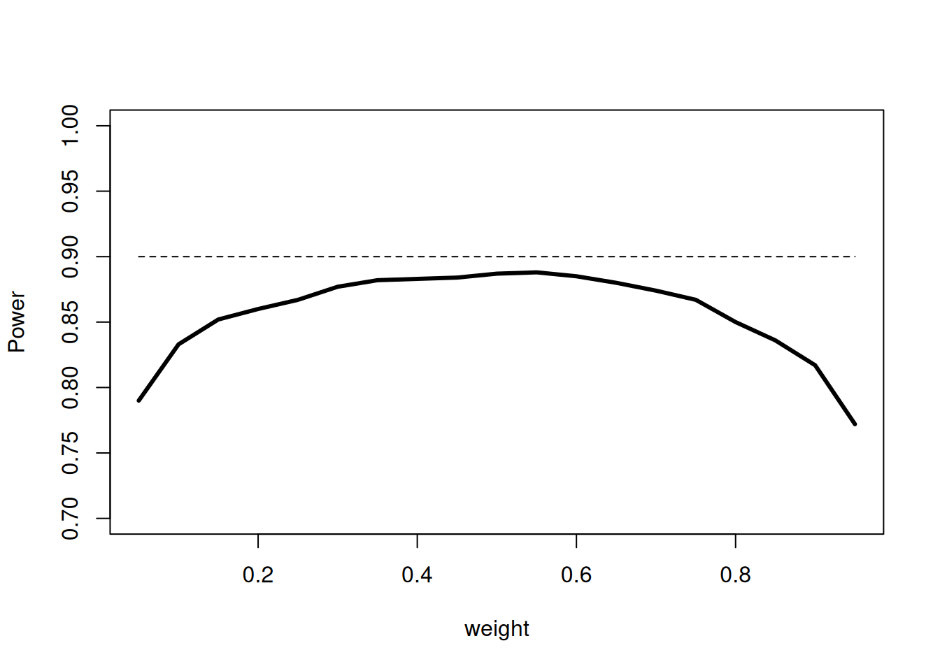
Assessing different selection rules
You might assess different selection rules by using the parameter typeOfSelection. Five options are available: best, rBest, epsilon, all, and userDefined. For rbest (select the r best treatment arms), the parameter rValue has to be specified, for epsilon (select treatment arm not worse than epsilon compared to the best), the parameter epsilonValue has to be specified.
User defined selection rule
If userDefined is selected, selectArmsFunction needs to be specified that depends on effectVector. Note that effectVector is either the test statistic or the effect difference (in absolute terms) which can be selected through the parameter effectMeasure. For example, using the function
designIN <- getDesignInverseNormal(kMax = 2, alpha = 0.025, typeOfDesign = "OF")
mySelectionFunction <- function(effectVector) {
    selectedArms <- (effectVector >= c(5, 5, 5))
    return(selectedArms)
}
defines a selection rule where all treatment arms with effect sizes exceeding 5 (with the default effectMeasure = effectEstimate) are selected. Running
simSelectionMAMS <- getSimulationMultiArmMeans(
    design = designIN,
    activeArms = 3,
    typeOfShape = "linear",
    muMaxVector = c(10),
    stDev = 15,
    plannedSubjects = c(30, 60),
    intersectionTest = "Dunnett",
    typeOfSelection = "userDefined",
    selectArmsFunction = mySelectionFunction,
    successCriterion = "atLeastOne",
    maxNumberOfIterations = maxNumberOfIterations,
    seed = 1234
)
kable(summary(simSelectionMAMS))
shows that for the second stage the expected number of selected treatment arms is 1.803 indicating that there are cases where more than one arm is selected for the second stage:
| stages | maxNumberOfIterations | seed | allocationRatioPlanned | futilityStop | stDev | plannedSubjects | activeArms | effectMatrix | typeOfShape | muMaxVector | slope | intersectionTest | typeOfSelection | effectMeasure | successCriterion | iterations | rejectAtLeastOne | futilityPerStage | earlyStop | successPerStage | numberOfActiveArms | expectedNumberOfSubjects | conditionalPowerAchieved |
|---|---|---|---|---|---|---|---|---|---|---|---|---|---|---|---|---|---|---|---|---|---|---|---|
| 1 | 1000 | 1234 | 1 | 0.07 | 15 | 30 | 3 | 10 | linear | 10 | 1 | Dunnett | userDefined | effectEstimate | atLeastOne | 1000 | 0.884 | 0.07 | 0.396 | 0.326 | 3.00000 | 170.79 | NA |
| 2 | 1000 | 1234 | 1 | 0.07 | 15 | 60 | 3 | 10 | linear | 10 | 1 | Dunnett | userDefined | effectEstimate | atLeastOne | 604 | 0.884 | NA | NA | 0.558 | 1.80298 | 170.79 | 0.4021222 |
Using getData() enables to show how often this is the case. The following code lines calculate how often 1, 2, and 3 treatment arms were selected for the second stage:
dat <- getData(simSelectionMAMS)
tab <- as.matrix(table(dat[dat$stageNumber == 2, ]$iterationNumber))
round(table(tab[, 1]) / nrow(tab), 5)
1 2 3 0.36258 0.47185 0.16556
Note that these probabilities are conditional probabilities (conditional on performing the second stage) and sum to one whereas the probabilities for selecting arm 1, 2, or 3 provided in the summary are unconditional, i.e., not conditioned on reaching the second stage. In particular, they may become small if the study often stops at interim.
epsilon selection rule
We now consider a three-stage inverse normal combination test design where no early stops for efficacy are foreseen. At the end, the full significance level of \(\alpha = 0.025\) should be used. This is achieved by the definition of the design through
designIN3Stages <- getDesignInverseNormal(
    typeOfDesign = "asUser",
    userAlphaSpending = c(0, 0, 0.025)
)
Changed type of design to 'noEarlyEfficacy'As above, we plan a design with three active treatment arms to be tested against control and assume a linear dose-response relationship. We want to consider a range of maximum values for the effect and therefore specify muMaxVector = seq(0,12,3), i.e., including the null hypothesis case. For the selection of treatment arms, we define the epsilon selection rule with \(\epsilon = 2\), i.e., for the subsequent stages, the treatment arm with the highest response and all treatment arms that differ less than 2 with the highest response are selected. To exclude treatment arms with non-positive response, we additionally specify threshold = 0. In order to simulate a situation with a maximum of 60 subject per treatment arm we set plannedSubjects = c(20, 40, 60):
simSelectionEpsilonMAMS <- getSimulationMultiArmMeans(
    design = designIN3Stages,
    activeArms = 3,
    typeOfShape = "linear",
    muMaxVector = seq(0, 12, 2),
    stDev = 15,
    plannedSubjects = c(20, 40, 60),
    intersectionTest = "Dunnett",
    typeOfSelection = "epsilon",
    epsilonValue = 2,
    threshold = 0,
    successCriterion = "atLeastOne",
    maxNumberOfIterations = maxNumberOfIterations,
    seed = 1234
)

options("rpact.summary.output.size" = "medium")
# kable(summary(simSelectionEpsilonMAMS))
kable(simSelectionEpsilonMAMS)| stages | maxNumberOfIterations | seed | allocationRatioPlanned | stDev | plannedSubjects | activeArms | effectMatrix | typeOfShape | muMaxVector | slope | intersectionTest | typeOfSelection | effectMeasure | successCriterion | epsilonValue | rValue | threshold | iterations | rejectAtLeastOne | futilityStop | futilityPerStage | earlyStop | successPerStage | numberOfActiveArms | expectedNumberOfSubjects | conditionalPowerAchieved |
|---|---|---|---|---|---|---|---|---|---|---|---|---|---|---|---|---|---|---|---|---|---|---|---|---|---|---|
| 1 | 1000 | 1234 | 1 | 15 | 20 | 3 | 0 | linear | 0 | 1 | Dunnett | epsilon | effectEstimate | atLeastOne | 2 | NA | 0 | 1000 | 0.023 | 0.355 | 0.241 | 0.241 | 0.000 | 3.000000 | 144.84 | NA |
| 1 | 1000 | 1234 | 1 | 15 | 20 | 3 | 2 | linear | 2 | 1 | Dunnett | epsilon | effectEstimate | atLeastOne | 2 | NA | 0 | 1000 | 0.079 | 0.235 | 0.165 | 0.165 | 0.000 | 3.000000 | 154.72 | NA |
| 1 | 1000 | 1234 | 1 | 15 | 20 | 3 | 4 | linear | 4 | 1 | Dunnett | epsilon | effectEstimate | atLeastOne | 2 | NA | 0 | 1000 | 0.216 | 0.108 | 0.075 | 0.075 | 0.000 | 3.000000 | 165.12 | NA |
| 1 | 1000 | 1234 | 1 | 15 | 20 | 3 | 6 | linear | 6 | 1 | Dunnett | epsilon | effectEstimate | atLeastOne | 2 | NA | 0 | 1000 | 0.475 | 0.066 | 0.053 | 0.053 | 0.000 | 3.000000 | 167.10 | NA |
| 1 | 1000 | 1234 | 1 | 15 | 20 | 3 | 8 | linear | 8 | 1 | Dunnett | epsilon | effectEstimate | atLeastOne | 2 | NA | 0 | 1000 | 0.720 | 0.024 | 0.021 | 0.021 | 0.000 | 3.000000 | 168.96 | NA |
| 1 | 1000 | 1234 | 1 | 15 | 20 | 3 | 10 | linear | 10 | 1 | Dunnett | epsilon | effectEstimate | atLeastOne | 2 | NA | 0 | 1000 | 0.899 | 0.008 | 0.006 | 0.006 | 0.000 | 3.000000 | 167.94 | NA |
| 1 | 1000 | 1234 | 1 | 15 | 20 | 3 | 12 | linear | 12 | 1 | Dunnett | epsilon | effectEstimate | atLeastOne | 2 | NA | 0 | 1000 | 0.968 | 0.004 | 0.004 | 0.004 | 0.000 | 3.000000 | 167.52 | NA |
| 2 | 1000 | 1234 | 1 | 15 | 40 | 3 | 0 | linear | 0 | 1 | Dunnett | epsilon | effectEstimate | atLeastOne | 2 | NA | 0 | 759 | 0.023 | 0.355 | 0.114 | 0.114 | 0.000 | 1.397892 | 144.84 | 0.0000000 |
| 2 | 1000 | 1234 | 1 | 15 | 40 | 3 | 2 | linear | 2 | 1 | Dunnett | epsilon | effectEstimate | atLeastOne | 2 | NA | 0 | 835 | 0.079 | 0.235 | 0.070 | 0.070 | 0.000 | 1.434730 | 154.72 | 0.0000000 |
| 2 | 1000 | 1234 | 1 | 15 | 40 | 3 | 4 | linear | 4 | 1 | Dunnett | epsilon | effectEstimate | atLeastOne | 2 | NA | 0 | 925 | 0.216 | 0.108 | 0.033 | 0.033 | 0.000 | 1.440000 | 165.12 | 0.0000000 |
| 2 | 1000 | 1234 | 1 | 15 | 40 | 3 | 6 | linear | 6 | 1 | Dunnett | epsilon | effectEstimate | atLeastOne | 2 | NA | 0 | 947 | 0.475 | 0.066 | 0.013 | 0.013 | 0.000 | 1.413939 | 167.10 | 0.0000000 |
| 2 | 1000 | 1234 | 1 | 15 | 40 | 3 | 8 | linear | 8 | 1 | Dunnett | epsilon | effectEstimate | atLeastOne | 2 | NA | 0 | 979 | 0.720 | 0.024 | 0.003 | 0.003 | 0.000 | 1.373851 | 168.96 | 0.0000000 |
| 2 | 1000 | 1234 | 1 | 15 | 40 | 3 | 10 | linear | 10 | 1 | Dunnett | epsilon | effectEstimate | atLeastOne | 2 | NA | 0 | 994 | 0.899 | 0.008 | 0.002 | 0.002 | 0.000 | 1.308853 | 167.94 | 0.0000000 |
| 2 | 1000 | 1234 | 1 | 15 | 40 | 3 | 12 | linear | 12 | 1 | Dunnett | epsilon | effectEstimate | atLeastOne | 2 | NA | 0 | 996 | 0.968 | 0.004 | 0.000 | 0.000 | 0.000 | 1.288153 | 167.52 | 0.0000000 |
| 3 | 1000 | 1234 | 1 | 15 | 60 | 3 | 0 | linear | 0 | 1 | Dunnett | epsilon | effectEstimate | atLeastOne | 2 | NA | 0 | 645 | 0.023 | 0.355 | NA | NA | 0.023 | 1.204651 | 144.84 | 0.1017799 |
| 3 | 1000 | 1234 | 1 | 15 | 60 | 3 | 2 | linear | 2 | 1 | Dunnett | epsilon | effectEstimate | atLeastOne | 2 | NA | 0 | 765 | 0.079 | 0.235 | NA | NA | 0.079 | 1.226144 | 154.72 | 0.1636927 |
| 3 | 1000 | 1234 | 1 | 15 | 60 | 3 | 4 | linear | 4 | 1 | Dunnett | epsilon | effectEstimate | atLeastOne | 2 | NA | 0 | 892 | 0.216 | 0.108 | NA | NA | 0.216 | 1.241031 | 165.12 | 0.2968530 |
| 3 | 1000 | 1234 | 1 | 15 | 60 | 3 | 6 | linear | 6 | 1 | Dunnett | epsilon | effectEstimate | atLeastOne | 2 | NA | 0 | 934 | 0.475 | 0.066 | NA | NA | 0.475 | 1.215203 | 167.10 | 0.4578361 |
| 3 | 1000 | 1234 | 1 | 15 | 60 | 3 | 8 | linear | 8 | 1 | Dunnett | epsilon | effectEstimate | atLeastOne | 2 | NA | 0 | 976 | 0.720 | 0.024 | NA | NA | 0.720 | 1.176230 | 168.96 | 0.6416432 |
| 3 | 1000 | 1234 | 1 | 15 | 60 | 3 | 10 | linear | 10 | 1 | Dunnett | epsilon | effectEstimate | atLeastOne | 2 | NA | 0 | 992 | 0.899 | 0.008 | NA | NA | 0.899 | 1.118952 | 167.94 | 0.8352505 |
| 3 | 1000 | 1234 | 1 | 15 | 60 | 3 | 12 | linear | 12 | 1 | Dunnett | epsilon | effectEstimate | atLeastOne | 2 | NA | 0 | 996 | 0.968 | 0.004 | NA | NA | 0.968 | 1.105422 | 167.52 | 0.9184243 |
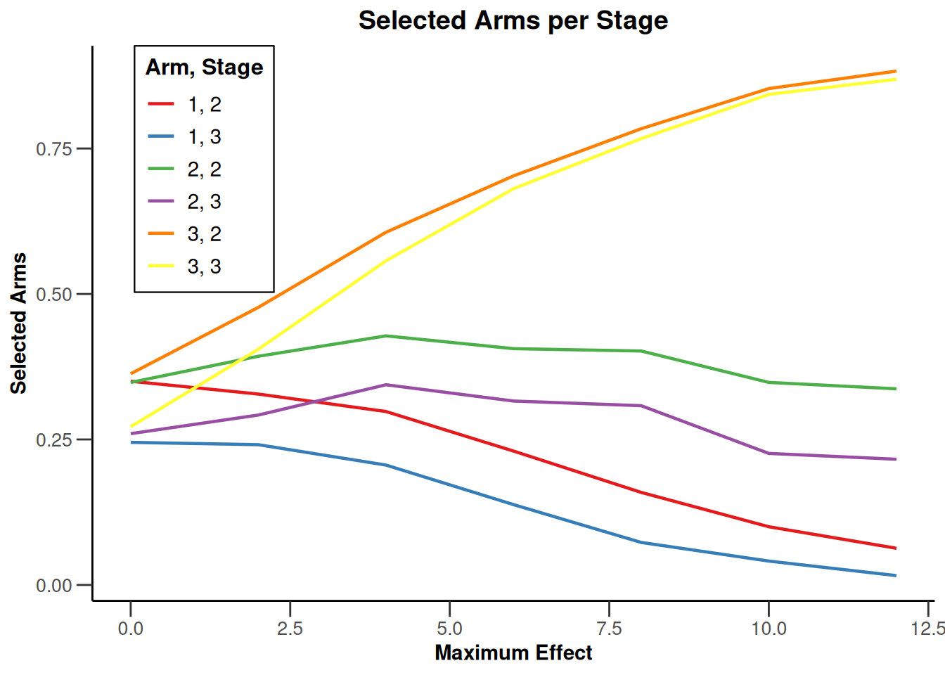
Note that we explicitly use the options("rpact.summary.output.size" = "medium") command because otherwise the output turns out to be too long. You might also illustrate the results through the generic plot command. For example, generating Overall Power/Early Stopping and Selected Arms per Stage plots are achieved by
plot(simSelectionEpsilonMAMS, type = c(5, 3), grid = 0)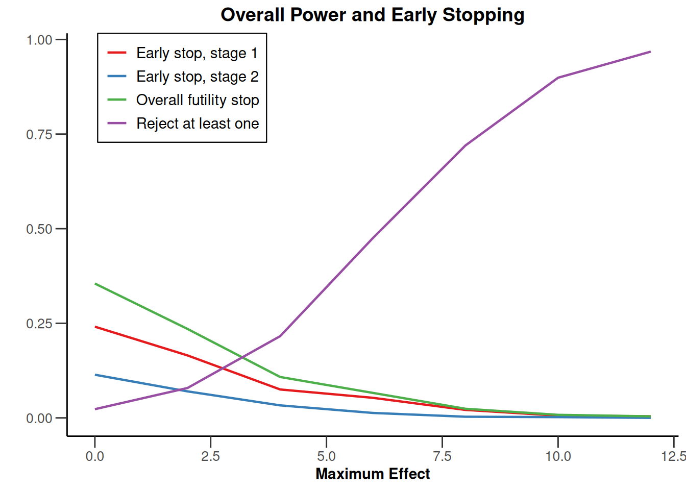
Closing remarks
This vignette can only give a brief introduction into possible configurations that can be considered within the simulation tool for multi-arm designs. Other than described here, for real-trial applications typically there is much more to take into account to adequately address the situation. For example, it might be of interest to additionally assess a sample size reassessment strategy. This can be performed as for simulating a single hypothesis situation (for example, see the vignette “Simulation of a trial with a binary endpoint and unblinded sample size re-calculation”).
For testing rates, the function getSimulationMultiArmRates() and for survival designs, the function getSimulationMultiArmSurvival() is available with very similar options as compared to the considered case. For survival designs, we note that - other than for the single hypothesis case - the function does not generate survival times on the subjects level, but normally distributed log-rank test statistics. As a consequence, for this case no estimates of analysis times, study duration, and expected number of subjects can be obtained.
System: rpact 4.0.0, R version 4.3.3 (2024-02-29 ucrt), platform: x86_64-w64-mingw32
To cite R in publications use:
R Core Team (2024). R: A Language and Environment for Statistical Computing. R Foundation for Statistical Computing, Vienna, Austria. https://www.R-project.org/. To cite package ‘rpact’ in publications use:
Wassmer G, Pahlke F (2024). rpact: Confirmatory Adaptive Clinical Trial Design and Analysis. R package version 4.0.0, https://www.rpact.com, https://github.com/rpact-com/rpact, https://rpact-com.github.io/rpact/, https://www.rpact.org.