library(dplyr)
library(ggplot2)
library(gridExtra)Enrichment Designs for Testing Rates with rpact
Planning
Rates
Analysis
Enrichment
This document provides examples for simulating test characteristics for multi-stage enrichment designs for testing rates with rpact. Specifically, it is shown how to obtain the simulation results for the example provided in Wassmer & Brannath (2016), Sect. 11.2. An example showing how to obtain results from a data analysis is provided too.
Summary
This document provides examples for simulating test characteristics for multi-stage enrichment designs for testing rates with rpact. Specifically, it is shown how to obtain the simulation results for the example provided in Wassmer & Brannath (2016), Sect. 11.2. An example showing how to obtain results from a data analysis is provided too.
Introduction
Adaptive enrichment designs are applicable in situations where studies of unselected patients might be unable to detect a drug effect and therefore it seems necessary to “enrich” the study with potential responders, defined as a subpopulation of the unselected patient population. If this is done in an adaptive and data-driven way (i.e., it is not clear upfront whether to use the selected population and this is decided based on data observed at an interim stage) we might use adaptive population enrichment designs.
Adaptive Enrichment Designs
Adaptive population enrichment designs enable the data-driven selection of one or more pre-specified subpopulations in an interim analysis and the confirmatory proof of efficacy in the selected subset(s) at the end of the trial. Sample size reassessment and other adaptive design changes can be performed as well. Strong control of the familywise error rate (FWER) is guaranteed by the use of \(p\)-value combination tests together with the closed testing principle.
Enrichment factors may be predictive biomarkers, or they may be biomarkers or clinicopathologic or demographic characteristics associated with a predictive biomarker or with the target of a therapeutic agent. The lower the proportion of truly benefiting patients, the more advantageous it is to consider studying an enriched population. However, instead of limiting the enrollment only to the narrow subpopulation of interest, prospectively specified adaptive designs may also be used to consider the effect of the experimental treatment both in the wider entire patient population under investigation and in various subpopulations.
Assume that there is a full population \(F\) with \(G - 1\) pre-specified subpopulations of interest denoted as \(S_1, S_2, \ldots, S_{G-1}\) such that \(S_g \subset F\). Let \(S_G\) denote the full population \(F\). Assume a binary endpoint and consider a set of \(G\) elementary hypotheses
\[ H_0^{S_g}: \pi_1^g = \pi_2^g, \; g = 1,\ldots,G, \]
where \(\pi_i^g\) denotes the unknown rates in treatment group \(i\), \(i=1,2\), and population \(g\), \(g = 1,\ldots,G\). That is, \(H_0^{S_g}\) refers to the response rate of the experimental treatment \(\pi_1^g\) versus control \(\pi_2^g\) in subpopulation \(S_g\).
At each stage \(k\), \(k=1,\ldots,K\), consider the test statistic
\[ Z^g=\frac{\hat\pi_1^g - \hat\pi_2^g}{\sqrt{\hat{\bar\pi}^g(1-\hat{\bar\pi}^g)}} \Big(\frac{1}{n_1^g}+\frac{1}{n_2^g}\Big)^{-1/2}, \]
where \(\hat\pi_1^g\) and \(\hat\pi_2^g\) are the observed rates at stage \(k\) in the two treatment groups and \(\hat{\bar\pi}^g = (n_1^g\hat\pi_1^g+n_2^g\hat\pi_2^g)/(n_1^g+n_2^g)\) is the observed cumulative rate in population \(S^g\) (at stage \(k\)). These test statistics are approximately normal and so the stage-wise \(p\,\)-values are calculated with the use of the normal cdf. If a subpopulation consists of several subsets, a stratified analysis should be performed where the corresponding Cochran-Mantel-Haenszel (CMH) test is applied.
The closed system of hypotheses consists of all possible intersection hypotheses
\[ H_0^{\cal J} = \bigcap_{g \in {\cal J}} H_0^{S_g}, \; {\cal J} \subseteq \{1,\ldots,G\}. \]
The global test decision follows from testing the global hypothesis
\[ H_0 = \bigcap_{g = 1}^G H_0^{S_g} \]
with a suitable global intersection test. If the global null hypothesis \(H_0\) can be rejected, all other intersection hypotheses are then tested. By performing the closed test procedure, an elementary hypothesis \(H_0^{S_g}\) can be rejected if the combination test fulfills the rejection criterion for all \(H_0^{\cal J}\) with \({\cal J} \ni g\).
Given a combination function \(C(\cdot,\cdot)\), at the second stage the hypothesis belonging to a selected subpopulation \(s\) is rejected if
\[ \min\limits_{{\cal J} \ni s} C(p_{{\cal J}},q_{{\cal J} \backslash {\cal E}}) \geq u_2\;, \]
where \({\cal E}\subset\{1,\ldots,G\}\) denotes the index set of all excluded \(H_0^g\), \({\cal J}\cap {\cal E}\not=\emptyset\), and \(u_2\) denotes the critical value for the second stage.
For \(G = 2\), using the adaptive closed test procedure, at an interim stage one can decide to continue to stage 2 to test \(H_0^F\) and \(H_0^S\), \(H_0^F\) only, or \(H_0^S\) only. Note that for a two-stage trial where no subpopulation is selected at interim, the complete set of intersection hypotheses is tested at each stage, yielding \(p\,\)-values \(p_{\cal J}\) and \(q_{\cal J}\) for each intersection hypothesis \(H_0^{\cal J}\). These \(p\,\)-values are combined according to the specified combination test, for example, the inverse normal method or Fisher’s combination test. This combination test might have a power disadvantage as compared to the single-stage non-adaptive test where the \(p\,\)-values would be obtained from the pooled data. However, we have the advantage that data-driven adaptations including subgroup selection are possible, thereby improving power.
The Simulation Function
First, load the R packages dplyr, ggplot2, and gridExtra:
Second, as always, load the rpact package:
library(rpact)
packageVersion("rpact") # should be version 3.3 or later
[1] '4.4.0.9305'The rpact function getSimulationEnrichmentRates() performs the simulation of a population enrichment design for testing the difference of proportions in two treatment groups. The way of how these simulations can be performed is similar to the case of multi-armed designs. Particularly, see the vignettes Planning and Analyzing a Group-Sequential Multi-Arm Multi-Stage Design with Binary Endpoint using rpact and Simulating Multi-Arm Designs with a Continuous Endpoint using rpact. Examples for creating plots for enrichment design simulations are illustrated in the vignette How to Create One- and Multi-Arm Simulation Result Plots with rpact.
An essentially new part required for enrichment designs is the definition of effect sizes and prevalences for the considered subpopulations. These typically consist of subsets of the considered entire (full) population (see Sect. 11.2 in Wassmer & Brannath, 2016).
For \(G = 2\), one subpopulation \(S\) is considered. Here, we have to specify the prevalence of \(S\) and the assumed effect sizes in \(S\) and \(R = F\backslash S\). The effect in \(F\) is a weighted average of the effect sizes in the disjoint subgroups \(S\) and \(R\), respectively. There is typically a large number of possible configurations because each effect size in \(S\) is combined with the effect sizes in \(R\). For \(G = 3\), things are more difficult. Generally, prevalences and effect sizes have to be specified for four subsets of \(F\) and even more possible configurations have to be considered. Note that also the case of nested or non-overlapping subpopulations can be considered as illustrated in Fig. 11.4 in Wassmer & Brannath (2016). rpact allows up to \(G = 4\), however, eight subsets need to be specified here.
In the rpact function getSimulationEnrichmentRates(), the parameter effectList has to be defined which is a list of parameters defining the subsets and yielding the subpopulations and their prevalences and effect sizes. We illustrate this for \(G = 2\) by the example presented in Wassmer & Dragalin (2015) and Wassmer & Brannath (2016), Sect. 11.2, and show how the results given there can be recalculated with the rpact function getSimulationEnrichmentRates().
A Simulation Trial Example
The study under consideration is the Investigation of Serial Studies to Predict Your Therapeutic Response with Imaging And moLecular Analysis (I-SPY 2 TRIAL) which is an ongoing clinical trial in patients with high-risk primary breast cancer. It involves a randomized phase II screening process in which a series of experimental drugs are evaluated in combination with standard neoadjuvant chemotherapy which is given prior to surgery. The primary endpoint is pathologic complete response (pCR) at the time of surgery (for details, see Barker et al., 2009).
The screening process includes a Magnetic Resonance Imaging to establish tumor size at baseline and a biopsy to identify the tumor’s hormone-receptor status (HR) and the HER2/neu status (HER2). Triple negative breast cancer (TNBC) refers to breast cancer that does not express the genes for the estrogen receptor, the progesterone receptor, and HER2.
Assume that one of the experimental drugs has been identified from I-SPY 2 TRIAL with the biomarker signature of TNBC but also with some promising effect in the HER2 negative (HER2-) biomarker signature. The sponsor may consider a confirmatory Phase III trial in TNBC patients only. The prevalence of TNBC, however, is only 34%, while the prevalence of HER2- is 63%. Therefore, an alternative option is to run a confirmatory trial with a two-stage enrichment design starting with the HER2- patients as the full population, but with the preplanned option of selecting the TNBC patients after the first stage if the observed effect is not promising in the HER2- patients with positive hormone-receptor status (HR+).
If a pCR rate in the control arm of 0.3 and a treatment effect of 0.2 (measured as the difference in pCR rates between the new drug and control) is assumed, the required total sample size for a conventional two-arm test with power 90% and one-sided significance level 0.0125 (i.e., applying Bonferroni correction) is 294. This can be found with rpact using the command
getSampleSizeRates(
    alpha = 0.0125,
    beta = 0.1,
    pi1 = 0.5,
    pi2 = 0.3)$nFixed |>
    ceiling()
[1] 294It will serve as a first guess for the actually needed sample size and we illustrate the enrichment design for this study assuming that a total sample size of 300 subjects will be enrolled in the trial.
The interim analysis is planned after 150 subjects and no early stopping is intended. The design under consideration therefore will be
designIN <- getDesignInverseNormal(
    kMax = 2,
    typeOfDesign = "noEarlyEfficacy"
)
A subpopulation selection using the \(\epsilon\)-selection rule with \(\epsilon = 0.1\) will be considered, i.e., if the difference in pCR is smaller than 0.1, both populations are selected and the decision at the interim analysis will be to either select the TNBC subpopulation or going on with the full population of HER2- patients. If the observed treatment effect difference exceeds 0.1 in favor of the TNBC population, the TNBC subpopulation will be selected, otherwise no selection will be considered. In this case, the test for the full population only will be conducted if the observed treatment effect difference exceeds 0.1 in favor of the F population; otherwise the test for both populations will be conducted. The inverse normal combination testing strategy together with the Simes intersection test will be used. We use the Simes test here to avoid futility stops that are possibly due to the use of the Bonferroni correction.
In I-SPY 1 TRIAL, a prevalence of TNBC patients in the HER2- population of about 54% (\(\approx 34/63\cdot 100\)%) and a control pCR rate in TNBC patients of 0.34 was observed. The control pCR rate in the HER2- patients with HR+ hormone receptor is 0.23. The operating characteristics of the enrichment design are investigated for treatment effect differences ranging from 0 to 0.3 by an increment of 0.05 in the TNBC subpopulation and ranging from 0 to 0.2 by an increment of 0.10 in the HER2- patients with HR+ hormone receptor. This yields 21 different scenarios for the effect sizes that are defined in the parameter list effectList as follows.
effectList <- list(
    subGroups = c("R", "S"),
    prevalences = c(0.46, 0.54),
    piControl = c(0.23, 0.34),
    piTreatments = expand.grid(
        seq(0, 0.2, 0.1) + 0.23,
        seq(0, 0.3, 0.05) + 0.34
    )
)
effectList
$subGroups
[1] "R" "S"
$prevalences
[1] 0.46 0.54
$piControl
[1] 0.23 0.34
$piTreatments
Var1 Var2
1 0.23 0.34
2 0.33 0.34
3 0.43 0.34
4 0.23 0.39
5 0.33 0.39
6 0.43 0.39
7 0.23 0.44
8 0.33 0.44
9 0.43 0.44
10 0.23 0.49
11 0.33 0.49
12 0.43 0.49
13 0.23 0.54
14 0.33 0.54
15 0.43 0.54
16 0.23 0.59
17 0.33 0.59
18 0.43 0.59
19 0.23 0.64
20 0.33 0.64
21 0.43 0.64We see that different situations as specified per row of piTreatments can be considered. For the above definition, using the specified prevalences, this yields the following 21 treatment effect differences for the full population \(F\) (see Table 11.3 in Wassmer & Brannath, 2016):
diffEffectsF <- effectList$piTreatments -
    matrix(rep(effectList$piControl, 21), ncol = 2, byrow = TRUE)
(diffEffectsF * matrix(rep(effectList$prevalences, 21), ncol = 2, byrow = TRUE)) |>
    rowSums() |> as.matrix()
[,1]
[1,] 0.000
[2,] 0.046
[3,] 0.092
[4,] 0.027
[5,] 0.073
[6,] 0.119
[7,] 0.054
[8,] 0.100
[9,] 0.146
[10,] 0.081
[11,] 0.127
[12,] 0.173
[13,] 0.108
[14,] 0.154
[15,] 0.200
[16,] 0.135
[17,] 0.181
[18,] 0.227
[19,] 0.162
[20,] 0.208
[21,] 0.254For the moment, we want to consider only one situation, namely
effectList <- list(
    subGroups = c("R", "S"),
    prevalences = c(0.46, 0.54),
    piControl = c(0.23, 0.34),
    piTreatments = c(0.43, 0.54)
)
That is, we consider the same effect difference (= 0.20) in each of the two subset, S and R. The design characteristics of 10,000 simulations are generated and summarized as follows:
getSimulationEnrichmentRates(
    design = designIN,
    plannedSubjects = c(150, 300),
    effectList = effectList,
    stratifiedAnalysis = TRUE,
    intersectionTest = "Simes",
    typeOfSelection = "epsilon",
    epsilonValue = 0.1,
    seed = 12345,
    maxNumberOfIterations = 10000
) |>
    summary()
Simulation of a binary endpoint (enrichment design)
Sequential analysis with a maximum of 2 looks (inverse normal combination test design), one-sided overall significance level 2.5%. The results were simulated for a population enrichment comparisons for rates (treatment vs. control, 2 populations), H0: pi(treatment) - pi(control) = 0, power directed towards larger values, H1: assumed pi(treatment) = c(0.54, 0.43), subgroups = c(S, R), prevalences = c(0.54, 0.46), control rates pi(control) = c(0.34, 0.23), planned cumulative sample size = c(150, 300), intersection test = Simes, selection = epsilon rule, eps = 0.1, effect measure based on effect estimate, success criterion: all, simulation runs = 500, seed = 12345.
| Stage | 1 | 2 |
|---|---|---|
| Fixed weight | 0.707 | 0.707 |
| Cumulative alpha spent | 0 | 0.0250 |
| Stage levels (one-sided) | 0 | 0.0250 |
| Efficacy boundary (z-value scale) | Inf | 1.960 |
| Reject at least one | 0.9160 | |
| Rejected populations per stage | ||
| Subset S | 0 | 0.7360 |
| Full population F | 0 | 0.8360 |
| Success per stage | 0 | 0.8020 |
| Stage-wise number of subjects | ||
| Subset S | 81.0 | 86.5 |
| Remaining population R | 69.0 | 63.5 |
| Expected number of subjects under H1 | 300.0 | |
| Overall exit probability | 0 | |
| Selected populations | ||
| Subset S | 1.0000 | 0.9280 |
| Full population F | 1.0000 | 0.9200 |
| Number of populations | 2.000 | 1.848 |
| Conditional power (achieved) | 0.7847 |
We see in Reject at least one that the power requirement is more or less exactly fulfilled and that there is a considerably higher chance to reject F. By default, successCriterion = "all" and therefore rejecting both populations, in this situation, has a probability of around 76%.
The design characteristics for the whole number of situations and 10,000 simulations per scenario are generated as follows:
effectList <- list(
    subGroups = c("R", "S"),
    prevalences = c(0.46, 0.54),
    piControl = c(0.23, 0.34),
    piTreatments = expand.grid(
        seq(0, 0.2, 0.1) + 0.23,
        seq(0, 0.3, 0.05) + 0.34
    )
)

simResultsPE <- designIN |>
    getSimulationEnrichmentRates(
        plannedSubjects = c(150, 300),
        effectList = effectList,
        stratifiedAnalysis = TRUE,
        intersectionTest = "Simes",
        typeOfSelection = "epsilon",
        epsilonValue = 0.1,
        seed = 12345,
        maxNumberOfIterations = 10000
    )
The results from Table 11.3 in Wassmer & Brannath (2016) are obtained from simResultsPE as follows:
simResultsPE$rejectAtLeastOne |> round(3) |> as.matrix() [,1]
[1,] 0.018
[2,] 0.076
[3,] 0.220
[4,] 0.082
[5,] 0.146
[6,] 0.406
[7,] 0.228
[8,] 0.414
[9,] 0.598
[10,] 0.450
[11,] 0.536
[12,] 0.758
[13,] 0.712
[14,] 0.784
[15,] 0.872
[16,] 0.876
[17,] 0.908
[18,] 0.968
[19,] 0.964
[20,] 0.976
[21,] 0.994simResultsPE$rejectedPopulationsPerStage[2, , ] |> round(3) [,1] [,2]
[1,] 0.014 0.016
[2,] 0.012 0.076
[3,] 0.024 0.218
[4,] 0.064 0.050
[5,] 0.082 0.126
[6,] 0.092 0.402
[7,] 0.202 0.108
[8,] 0.258 0.364
[9,] 0.232 0.584
[10,] 0.428 0.172
[11,] 0.434 0.386
[12,] 0.430 0.708
[13,] 0.698 0.212
[14,] 0.706 0.588
[15,] 0.658 0.766
[16,] 0.870 0.276
[17,] 0.862 0.568
[18,] 0.850 0.834
[19,] 0.962 0.226
[20,] 0.968 0.484
[21,] 0.954 0.768simResultsPE$selectedPopulations[2, , ] |> round(3) [,1] [,2]
[1,] 0.934 0.948
[2,] 0.782 0.988
[3,] 0.598 0.992
[4,] 0.974 0.872
[5,] 0.862 0.956
[6,] 0.666 0.994
[7,] 0.994 0.792
[8,] 0.930 0.930
[9,] 0.810 0.980
[10,] 0.992 0.666
[11,] 0.972 0.830
[12,] 0.852 0.946
[13,] 0.996 0.520
[14,] 0.980 0.808
[15,] 0.930 0.894
[16,] 0.998 0.424
[17,] 0.986 0.674
[18,] 0.950 0.868
[19,] 1.000 0.278
[20,] 0.998 0.522
[21,] 0.978 0.774The probability to select one population is obtained from numberOfPopulations through
P(select one population) + 2 * (1 - P(select one population)) = numberOfPopulations:
(2 - simResultsPE$numberOfPopulations[2, ]) |> round(3) |> as.matrix() [,1]
[1,] 0.118
[2,] 0.230
[3,] 0.410
[4,] 0.154
[5,] 0.182
[6,] 0.340
[7,] 0.214
[8,] 0.140
[9,] 0.210
[10,] 0.342
[11,] 0.198
[12,] 0.202
[13,] 0.484
[14,] 0.212
[15,] 0.176
[16,] 0.578
[17,] 0.340
[18,] 0.182
[19,] 0.722
[20,] 0.480
[21,] 0.248Note that the as.matrix() command used for the power (rejectAtLeastOne) and numberOfPopulations is only employed for better readability and is not essential.
The power of the design (the probability to reject at least one null hypothesis) is greater than 90% for scenarios 17-21, mainly corresponding to treatment effects 0.25 and 0.3 for \(S\). Hence, in these cases a total sample size of 300 patients reaches the desired power, and the rough estimate gathered above through the use of the Bonferroni correction provides a good estimate for the necessary sample size. Note that the term power is used here also for the cases where the null hypothesis is true (Scenarios 1-3). This, however, illustrates strong control of FWER (see the first three values of rejectedPopulationsPerStage[2, ,1]). Note that in the records, the first column refers to S, whereas the second refers to F.
The results also show that the power to reject in the full population (except for effect size \(\geq 0.2\) and \(< 0.3\) in both subsets, i.e., scenarios 15 and 18) is smaller than 80%, for largest effect sizes the power even decreases a bit. The latter is due to the fact that in this case, the probability to deselect \(F\) and to select \(S\) increases. For most scenarios the probability to reduce the confirmatory proof to one hypothesis, \(H_0^S\) or \(H_0^F\), is quite small.
The probability for enrichment, i.e., the selection of \(S\) at the interim stage, varies between 1% and 70% over the scenarios and can be derived from P(Select \(F\)) = selectedPopulations[2, ,2] as P(Enrichment) = 1 - P(Select \(F\)).
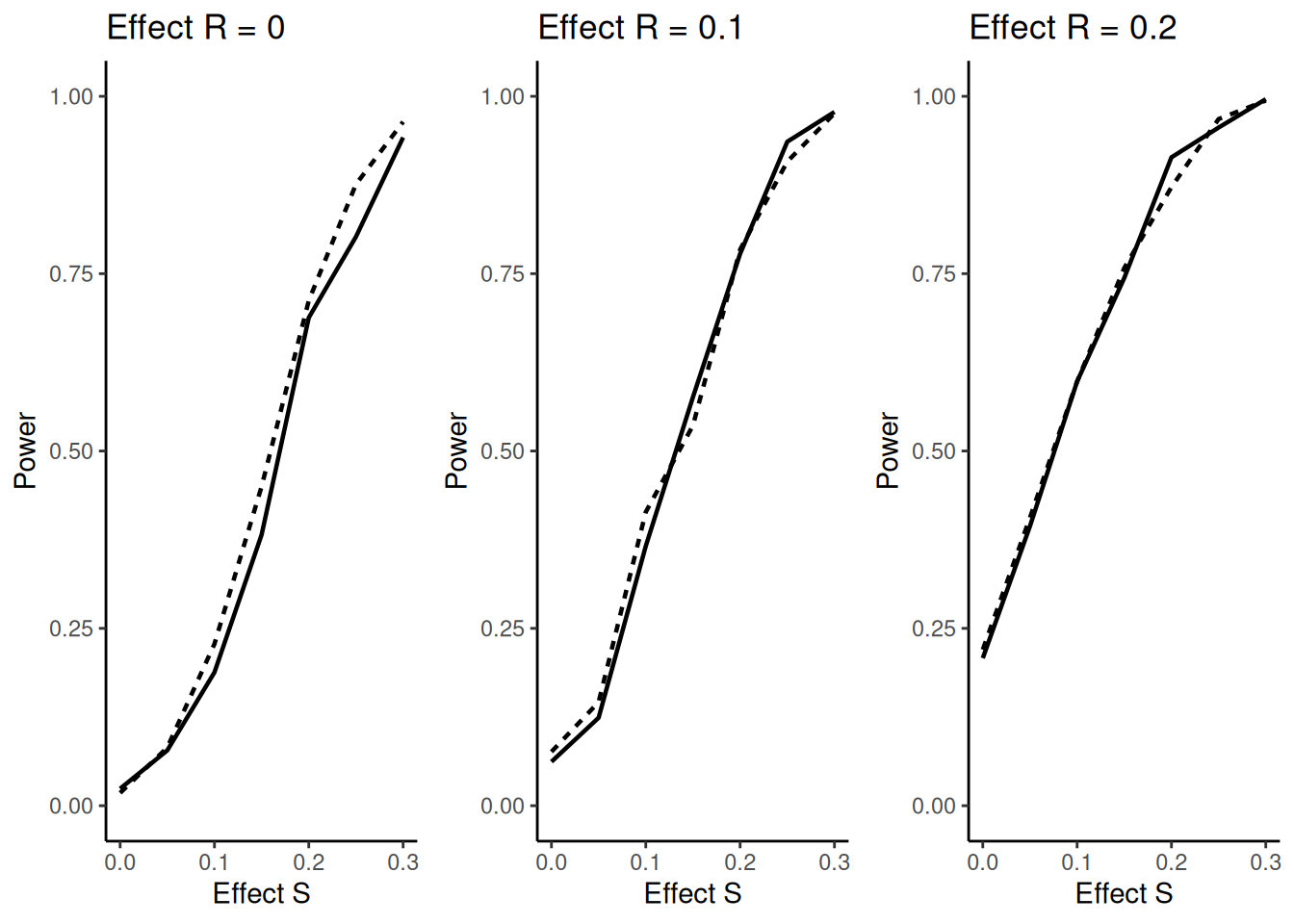
The question arises if this might reduce power (defined as above) due to wrongly selecting a population. The answer is no, as illustrated in the figure below. Here it is shown that for all effect sizes in \(\bar S = R\) there is no decrease, for effect size 0 there is even a clear increase in power showing the advantage of an adaptive enrichment design as compared to the non-adaptive case. In the figure, the dashed lines refer to the cases with selection and the solid lines to the non-adaptive case.
The following code is used to create the plots above:
simResultsFixed <- getSimulationEnrichmentRates(
    design = designIN,
    plannedSubjects = c(150, 300),
    effectList = effectList,
    stratifiedAnalysis = TRUE,
    intersectionTest = "Simes",
    typeOfSelection = "all",
    seed = 12345,
    maxNumberOfIterations = 10000
)

dataAll <- rbind(
    simResultsFixed |> as.data.frame(),
    simResultsPE |> as.data.frame()
)
dataAll$effectS <- effectList$piTreatments$Var2 - effectList$piControl[2]
dataAll$effectNotS <- (effectList$piTreatments$Var1 - effectList$piControl[1]) |>
    round(1)

dataStage2 <- dataAll |>
    filter(stages == 2)

plotPowerDiff <- function(effectR) {
    dataSub <- dataStage2 |>
        filter(effectNotS == effectR)
    ggplot(
        dataSub,
        aes(
            x = effectS, y = rejectAtLeastOne,
            group = typeOfSelection,
            linetype = typeOfSelection
        )
    ) +
        geom_line(linewidth = 0.8, show.legend = FALSE) +
        ylim(0, 1) +
        theme_classic() +
        xlab("Effect S") +
        ylab("Power") +
        ggtitle(paste0("Effect R = ", effectR))
}
plot1 <- plotPowerDiff(effectR = 0)
plot2 <- plotPowerDiff(effectR = 0.1)
plot3 <- plotPowerDiff(effectR = 0.2)

gridExtra::grid.arrange(plot1, plot2, plot3, ncol = 3)
Note that the definition of subGroups in the list determines how many and which type of subpopulations is considered for the clinical trial situation. In rpact, up to four subpopulations can be considered:
For \(G = 3\), subGroups with (fixed) names “R”,“S1”, “S2”, and “S12” have to be specified, i.e.,
subGroups = c("R", "S1", "S2", "S12")
and prevalences, piControl and piTreatments consist of four elements per situation.
For \(G = 4\), subGroups with (fixed) names “R”,“S1”, “S2”, “S2”, “S12”, “S13” “S23” and “S123” have to be specified, i.e.,
subGroups = c("R","S1", "S2", "S3", "S12", "S13", "S23", "S123")
and prevalences, piControl and piTreatments consist of eight elements per situation.
A Data Analysis Example
For a binary endpoint, the calculation of the test statistics and related computations for the test procedure require the number of events and the sample sizes. In rpact, these can be simply specified through separate data sets for the distinct subsets, S and R. For example, assume the results for the first and the second stage in the two subsets are as follows:
S <- getDataSet(
    events1 = c(11, 12),
    events2 = c(6, 7),
    n1 = c(36, 39),
    n2 = c(38, 40)
)

R <- getDataSet(
    events1 = c(12, 10),
    events2 = c(8, 8),
    n1 = c(32, 33),
    n2 = c(31, 29)
)

F <- getDataSet(
    events1 = c(23, 22),
    events2 = c(14, 15),
    n1 = c(68, 72),
    n2 = c(69, 69)
)
The whole data set and the analysis with Simes’ test is then obtained with
designIN |>
    getDataSet(S1 = S, R = R) |>
    getAnalysisResults(intersectionTest = "Simes") |>
    summary()
Enrichment analysis results for a binary endpoint (2 populations)
Sequential analysis with 2 looks (inverse normal combination test design), one-sided overall significance level 2.5%. The results were calculated using a two-sample test for rates, Simes intersection test, normal approximation test, stratified analysis. H0: pi(treatment) - pi(control) = 0 against H1: pi(treatment) - pi(control) > 0.
| Stage | 1 | 2 |
|---|---|---|
| Fixed weight | 0.707 | 0.707 |
| Cumulative alpha spent | 0 | 0.0250 |
| Stage levels (one-sided) | 0 | 0.0250 |
| Efficacy boundary (z-value scale) | Inf | 1.960 |
| Cumulative effect size S1 | 0.148 | 0.140 |
| Cumulative effect size F | 0.135 | 0.111 |
| Cumulative treatment rate S1 | 0.306 | 0.307 |
| Cumulative treatment rate F | 0.338 | 0.321 |
| Cumulative control rate S1 | 0.158 | 0.167 |
| Cumulative control rate F | 0.203 | 0.210 |
| Stage-wise test statistic S1 | 1.509 | 1.380 |
| Stage-wise test statistic F | 1.768 | 1.167 |
| Stage-wise p-value S1 | 0.0656 | 0.0838 |
| Stage-wise p-value F | 0.0385 | 0.1217 |
| Adjusted stage-wise p-value S1, F | 0.0656 | 0.1217 |
| Adjusted stage-wise p-value S1 | 0.0656 | 0.0838 |
| Adjusted stage-wise p-value F | 0.0385 | 0.1217 |
| Overall adjusted test statistic S1, F | 1.509 | 1.892 |
| Overall adjusted test statistic S1 | 1.509 | 2.043 |
| Overall adjusted test statistic F | 1.768 | 2.075 |
| Test action: reject S1 | FALSE | FALSE |
| Test action: reject F | FALSE | FALSE |
| Conditional rejection probability S1 | 0.1034 | |
| Conditional rejection probability F | 0.1034 | |
| 95% repeated confidence interval S1 | [-0.029; 0.306] | |
| 95% repeated confidence interval F | [-0.021; 0.238] | |
| Repeated p-value S1 | 0.0292 | |
| Repeated p-value F | 0.0292 |
Legend:
- F: full population
- S[i]: population i
From the first stage, it is seen that the effect differences between S and R, and hence between S and F, are quite similar. Following the \(\epsilon\)-selection rule with \(\epsilon = 0.1\), and since 11/36 - 6/38 = 0.148 and 23/68 - 14/69 = 0.135, no enrichment was performed and both subsets were used in the second stage. After both stages are observed, however, none of the hypotheses can be rejected. As an exercise, the reader is encouraged to verify that the use of the Spiessens and Debois test yields an only negligibly smaller overall \(p\)-value ( = 0.0288) that does not reach significance either. However, the Bonferroni test is considerably worse yielding an overall \(p\)-value of 0.0456.
As an alternative, one might consider the case of enrichment, i.e., to decide at interim to proceed with the trial with the subset S only. The sample size for the second stage can be chosen in a data-driven manner. Because of
designIN |>
    getDataSet(S1 = S, R = R) |>
    getAnalysisResults(
        stage = 1,
        nPlanned = 150,
        intersectionTest = "Simes"
    ) |>
    fetch(conditionalPower)
$conditionalPower
[,1] [,2]
[1,] NA 0.8144225
[2,] NA 0.7290993the conditional power when sticking to the originally planned sample size is large enough (> 80%) for the rejection of the hypothesis for subset S and hence, it might be decided to recruit patients from S only. Assume that the following observations were made:
S <- getDataSet(
    events1 = c(11, 46),
    events2 = c(6, 27),
    n1 = c(36, 151),
    n2 = c(38, 148)
)

R <- getDataSet(
    events1 = c(12, NA),
    events2 = c(8, NA),
    n1 = c(32, NA),
    n2 = c(31, NA)
)
This is the result showing clear significance of an effect in S although the observed effect is virtually the same as before:
designIN |>
    getDataSet(S1 = S, R = R) |>
    getAnalysisResults(intersectionTest = "Simes") |>
    summary()
Enrichment analysis results for a binary endpoint (2 populations)
Sequential analysis with 2 looks (inverse normal combination test design), one-sided overall significance level 2.5%. The results were calculated using a two-sample test for rates, Simes intersection test, normal approximation test, stratified analysis. H0: pi(treatment) - pi(control) = 0 against H1: pi(treatment) - pi(control) > 0.
| Stage | 1 | 2 |
|---|---|---|
| Fixed weight | 0.707 | 0.707 |
| Cumulative alpha spent | 0 | 0.0250 |
| Stage levels (one-sided) | 0 | 0.0250 |
| Efficacy boundary (z-value scale) | Inf | 1.960 |
| Cumulative effect size S1 | 0.148 | 0.127 |
| Cumulative effect size F | 0.135 | |
| Cumulative treatment rate S1 | 0.306 | 0.305 |
| Cumulative treatment rate F | 0.338 | |
| Cumulative control rate S1 | 0.158 | 0.177 |
| Cumulative control rate F | 0.203 | |
| Stage-wise test statistic S1 | 1.509 | 2.459 |
| Stage-wise test statistic F | 1.768 | |
| Stage-wise p-value S1 | 0.0656 | 0.0070 |
| Stage-wise p-value F | 0.0385 | |
| Adjusted stage-wise p-value S1, F | 0.0656 | 0.0070 |
| Adjusted stage-wise p-value S1 | 0.0656 | 0.0070 |
| Adjusted stage-wise p-value F | 0.0385 | |
| Overall adjusted test statistic S1, F | 1.509 | 2.806 |
| Overall adjusted test statistic S1 | 1.509 | 2.806 |
| Overall adjusted test statistic F | 1.768 | |
| Test action: reject S1 | FALSE | TRUE |
| Test action: reject F | FALSE | FALSE |
| Conditional rejection probability S1 | 0.1034 | |
| Conditional rejection probability F | 0.1034 | |
| 95% repeated confidence interval S1 | [0.025; 0.239] | |
| 95% repeated confidence interval F | ||
| Repeated p-value S1 | 0.0025 | |
| Repeated p-value F |
Legend:
- F: full population
- S[i]: population i
References
Barker, A., Sigman, C., Kelloff, G., Hylton, N., Berry, D., Esserman, L. (2009). I–SPY 2: An adaptive breast cancer trial design in the setting of neoadjuvant chemotherapy. Clinical Pharmacology and Therapeutics 86, 97–100. https://doi.org/10.1038/clpt.2009.68
Wassmer, G and Brannath, W. Group Sequential and Confirmatory Adaptive Designs in Clinical Trials (2016), ISBN 978-3319325606 https://doi.org/10.1007/978-3-319-32562-0
Wassmer, G., Dragalin, V. (2015). Designing issues in confirmatory adaptive population enrichment trials. Journal of Biopharmaceutical Statistics 25, 651–669. https://doi.org/10.1080/10543406.2014.920869
System rpact 4.4.0.9305, R version 4.6.0 (2026-04-24), platform x86_64-pc-linux-gnu
To cite R in publications use:
R Core Team (2026). R: A Language and Environment for Statistical Computing. R Foundation for Statistical Computing, Vienna, Austria. doi:10.32614/R.manuals https://doi.org/10.32614/R.manuals. https://www.R-project.org/.
To cite package ‘rpact’ in publications use:
Wassmer G, Pahlke F (2026). rpact: Confirmatory Adaptive Clinical Trial Design and Analysis. R package version 4.4.0.9305. doi:10.32614/CRAN.package.rpact
Wassmer G, Brannath W (2025). Group Sequential and Confirmatory Adaptive Designs in Clinical Trials, 2nd edition. Springer, Cham, Switzerland. ISBN 978-3-031-89668-2. doi:10.1007/978-3-031-89669-9 https://doi.org/10.1007/978-3-031-89669-9.