Delayed Response Designs with rpact
Planning
This document provides a brief introduction to group sequential designs with delayed responses as proposed by Hampson and Jennison (2013). It is shown how this is implemented in rpact. Examples for designing trials with delayed responses using the software are provided. We also describe an alternative approach that directly uses the \(\alpha\)-spending approach to derive the decision boundaries.
Introduction
In rpact version 3.3, the group sequential methodology from Hampson and Jennison (2013) is implemented. As traditional group sequential designs are characterized specifically by the underlying boundary sets, one main task was to write a function returning the decision critical values according to the calculation rules in Hampson and Jennison (2013). The function returning the respective critical values has been validated, particularly via simulation towards Type I error rate control in various settings (for an example see below). Subsequently, functions characterizing a delayed response group sequential test in terms of power, maximum sample size and expected sample size have been written. These functions were integrated in the rpact functions getDesignGroupSequential(), getDesignCharacteristics(), and the corresponding getSampleSize...() and getPower...() functions.
Methodology
The classical group sequential methodology works on the assumptions of having no treatment response delay, i.e., it is assumed that enrolled subjects are observed upon recruitment or at least shortly after. In many practical situations, this assumption does not hold true. Instead, it might be that there is a latency between the timing of recruitment and the actual measurement of a primary endpoint. That is, at interim \(k\) there is some information \(I_{\Delta_t, k} > 0\) in pipeline.
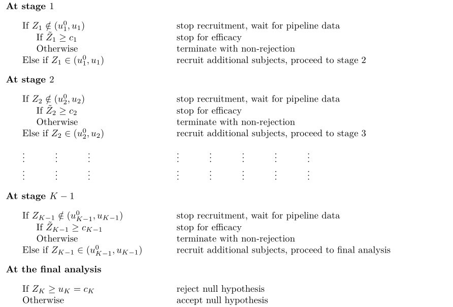
One method to handle this pipeline information was proposed by Hampson & Jennison (2013) and is called delayed response group sequential design. Assume that, in a \(K\)-stage trial, given we will proceed to the trial end, we will observe an information sequence \((I_1, \dots, I_K)\), and the corresponding \(Z\)-statistics \((Z_1, \dots, Z_K)\). As we now have information in pipeline, define \(\tilde{I}_k = I_k + I_{\Delta_t, k}\) as the information available after awaiting the delay after having observed \(I_k\). Let \((\tilde{Z}_1,\dots,\tilde{Z}_{K-1})\) be the vector of \(Z\)-statistics that are calculated based upon the information levels \((\tilde{I}_1,\dots,\tilde{I}_{K-1})\). Given boundary sets \(\{u^0_1,\dots,u^0_{K-1}\}\), \(\{u_1,\dots,u_K\}\) and \(\{c_1,\dots,c_K\}\), a \(K\)-stage delayed response group sequential design has the following structure:
That is, at each of the \(k=1,\dots,K-1\) interim analyses, there is \(I_{\Delta_t, k}\) information outstanding. If \(Z_k\) does not fall within \((u^0_k, u_k)\), the conclusion is to stop the trial neither for efficacy nor for futility (as it would be in a traditional group sequential design), but to irreversibly stop the recruitment. Afterwards, the outstanding data is awaited such that after awaiting the delayed information fraction \(I_{\Delta_t, k}\) of time, \(\tilde{I}_k := I_k + I_{\Delta_t, k}\) information is available and a new \(Z\)-statistic \(\tilde{Z}_k\) can be calculated. This statistic is then used to test the actual hypothesis of interest using a decision critical value \(c_k\). The heuristic idea is that the recruitment is stopped only if one is “confident about the subsequent decision”. This means that if the recruitment has been stopped for \(Z_k \geq u_k\), it should be likely to obtain a subsequent \(H_0\) rejection. In contrast, if the recruitment is stopped for \(Z_k \leq u^0_k\), obtaining a subsequent rejection should be rather unlikely (but still possible).
The main difference to a group sequential design is that due to the delayed information, each interim potentially consists of two analyses: a recruitment stop analysis and, if indicated, a subsequent decision analysis. Hampson & Jennison (2013) propose to define the boundary sets \(\{u^0_1,\dots,u^0_K\}\) and \(\{u_1,\dots,u_K\}\) as error-spending boundaries determined using \(\alpha\)-spending and \(\beta\)-spending functions in the one-sided testing setting with binding futility boundaries. In rpact, this methodology is extended to (one-sided) testing situations where (binding or non-binding) futility boundaries are available. According to Hampson & Jennison (2013), the boundaries \(\{c_1, \dots, c_K\}\) with \(c_K = u_K\) are chosen such that “reversal probabilities” are balanced. More precisely, \(c_1\) is chosen as the (unique) solution of:
\[\begin{align}\label{fs:delayedResponseCondition1} P_{H_0}(Z_1 \geq u_1, \tilde{Z}_1 < c_1) = P_{H_0}(Z_1 \leq u^0_1, \tilde{Z}_1 \geq c_1) \end{align}\]
and for \(k=2,\dots,K-1\), \(c_k\) is the (unique) solution of:
\[\begin{align}\label{fs:delayedResponseCondition2} \begin{split} &P_{H_0}(Z_1 \in (u^0_1, u_1), \dots, Z_{k-1} \in (u^0_{k-1}, u_{k-1}), Z_k \geq u_k, \tilde{Z}_k \leq c_k) \\ &= P_{H_0}(Z_1 \in (u^0_1, u_1), \dots, Z_{k-1} \in (u^0_{k-1}, u_{k-1}), Z_k \leq u^0_k, \tilde{Z}_k \geq c_k). \end{split} \end{align}\]
It can easily be shown that this constraint yields critical values that ensure Type I error rate control. We call this approach the reverse probabilities approach.
The values \(c_k\), \(k = 1,\ldots,K-1\), are determined via a root-search. Having determined all applicable boundaries, the rejection probability of the procedure given a treatment effect \(\delta\) is:
\[\begin{align}\label{fs:delayedResponsePower} \begin{split} P_{\delta}(Z_1 &\notin (u^0_1, u_1), \tilde{Z}_1 > c_1) \\ &+ \sum_{k=2}^{K-1} P_{\delta}(Z_1 \in (u^0_1, u_1), \dots , Z_{k-1} \in (u^0_{k-1}, u_{k-1}), Z_k \notin (u^0_k, u_k), \tilde{Z}_k \geq c_k) \\ &+ P_{\delta}(Z_1 \in (u^0_1, u_1), \dots , Z_{K-1} \in (u^0_{K-1}, u_{K-1}), Z_K \geq c_K)\,, \end{split} \end{align}\]
i.e., the probability to firstly stop the recruitment, followed by a rejection at any of the \(K\) stages. Setting \(\delta=0\), this expression gives the Type I error rate. These values are calculated also for \(\delta\not= 0\) and specified maximum sample size \(N\) (in the prototype case of testing \(H_0: \mu = 0\) against \(H_1:\mu = \delta\) with \(\sigma = 1\)).
As for the group sequential designs, the inflation factor, \(\widetilde{IF}\), of a delayed response design is the maximum sample size, \(\tilde N\), to achieve power \(1 - \beta\) for testing \(H_0\) against \(H_1\) (in the prototype case) relative to the fixed sample size, \(n_{fix}\):
\[\begin{equation}\label{fs:delayedResponseInflationFactor} \widetilde{IF} = \widetilde{IF}(\alpha, \beta, K , I_{\Delta_t}) = \frac{\widetilde N}{n_{fix}}\;. \end{equation}\]
Let \(n_k\) denote the number of subjects observed at the \(k\)-th recruitment stop analysis and \(\tilde{n}_k\) the number of subjects recruited at the subsequent \(k\)-th decision analysis. Given \(\widetilde N\), it holds that
\[\begin{align}\label{fs:delayedResponseSampleSize} n_k = I_k \widetilde N \,\,\,\, \text{and} \,\,\,\, \tilde{n}_k = \tilde{I}_k \widetilde N \;. \end{align}\]
The expected sample size, \(\widetilde{ASN}_\delta\), of a delayed response design is:
\[\begin{align}\label{fs:delayedResponseASN} \begin{split} \widetilde{ASN}_{\delta} = \tilde{n}_1 &P_{\delta}(Z_1 \notin (u^0_1, u_1)) \\ &+ \sum_{k=2}^{K-1} \tilde{n}_kP_{\delta}(Z_1 \in (u^0_1, u_1), \dots , Z_{k-1} \in (u^0_{k-1}, u_{k-1}), Z_k \notin (u^0_k, u_k)) \\ &+ \tilde{n}_K P_{\delta}(Z_1 \in (u^0_1, u_1), \dots , Z_{K-1} \in (u^0_{K-1}, u_{K-1})) \end{split} \end{align}\]
with \(\tilde{n}_K = \widetilde N\). As for the maximum sample size, this is provided relative to the sample size in a fixed sample design, i.e., as the expected reduction in sample size.
Examples
We illustrate the calculation of decision critical values and design characteristics using the described approach for a three-stage group sequential design with Kim & DeMets \(\alpha\)- and \(\beta\)-spending functions with \(\gamma = 2\).
First, load the rpact package
library(rpact)
packageVersion("rpact") # version should be version 3.3 or later
[1] '4.4.0.9305'Decision critical values
The delayed responses utility is simply to add the parameter delayedInformation to the getDesignGroupSequential() (or getDesignInverseNormal()) function. delayedInformation is either a positive constant or a vector of length \(K-1\) with positive elements describing the amount of pipeline information at interim \(k,\ldots,K-1\):
gsdWithDelay <- getDesignGroupSequential(
    kMax = 3,
    alpha = 0.025,
    beta = 0.2,
    typeOfDesign = "asKD",
    gammaA = 2,
    gammaB = 2,
    typeBetaSpending = "bsKD",
    informationRates = c(0.3, 0.7, 1),
    delayedInformation = c(0.16, 0.2),
    bindingFutility = TRUE
)
Note that the entered informationRates correspond to the information rates at which the decision to potentially stop recruitment is made (i.e., using the notation above, \(I_1,...,I_{K-1}\) for the interim analyses) rather than the information rates achieved at the efficacy decision (which are, in contrast, \(\tilde{I}_1,...\tilde{I}_{K-1}\)).
The output contains the continuation region for each interim analysis defined through the upper and lower boundary of the continuation region. The interim analyses are additionally characterized through decision critical values (1.387, 1.82, 2.03):
gsdWithDelayDesign parameters and output of group sequential design
User defined parameters
- Type of design: Kim & DeMets alpha spending
- Information rates: 0.300, 0.700, 1.000
- Binding futility: TRUE
- Parameter for alpha spending function: 2
- Parameter for beta spending function: 2
- Delayed information: 0.160, 0.200
- Type of beta spending: Kim & DeMets beta spending
Derived from user defined parameters
- Maximum number of stages: 3
Default parameters
- Stages: 1, 2, 3
- Significance level: 0.0250
- Type II error rate: 0.2000
- Test: one-sided
- Tolerance: 0.00000001
Output
- Power: 0.1053, 0.5579, 0.8000
- Lower bounds of continuation (binding): -0.508, 1.096
- Cumulative alpha spending: 0.00225, 0.01225, 0.02500
- Cumulative beta spending: 0.0180, 0.0980, 0.2000
- Upper bounds of continuation: 2.841, 2.295, 2.030
- Stage levels (one-sided): 0.00225, 0.01087, 0.02116
- Decision critical values: 1.387, 1.820, 2.030
- Reversal probabilities: 0.00007335, 0.00179791
Note that the last decision critical value (2.03) is equal to the last critical value of the corresponding group sequential design without delayed response. To obtain the design characteristics, the function getDesignCharacteristics() calculates the maximum sample size for the design (shift), the inflation factor and the average sample sizes under the null hypothesis, the alternative hypothesis, and under a value in between \(H_0\) and \(H_1\):
gsdWithDelay |> getDesignCharacteristics()Delayed response group sequential design characteristics
- Number of subjects fixed: 7.8489
- Shift: 8.2521
- Inflation factor: 1.0514
- Informations: 2.476, 5.777, 8.252
- Power: 0.1026, 0.5563, 0.8000
- Rejection probabilities under H1: 0.1026, 0.4537, 0.2437
- Futility probabilities under H1: 0.01869, 0.08335
- Ratio expected vs fixed sample size under H1: 0.9269
- Ratio expected vs fixed sample size under a value between H0 and H1: 0.9329
- Ratio expected vs fixed sample size under H0: 0.8165
Using the summary() function, these number can be directly displayed without using the getDesignCharacteristics() function as follows:
gsdWithDelay |> summary()Sequential analysis with a maximum of 3 looks (delayed response group sequential design)
Kim & DeMets alpha spending design with delayed response (gammaA = 2) and Kim & DeMets beta spending (gammaB = 2), one-sided overall significance level 2.5%, power 80%, undefined endpoint, inflation factor 1.0514, ASN H1 0.9269, ASN H01 0.9329, ASN H0 0.8165.
| Stage | 1 | 2 | 3 |
|---|---|---|---|
| Planned information rate | 30% | 70% | 100% |
| Delayed information | 16% | 20% | |
| Cumulative alpha spent | 0.0022 | 0.0122 | 0.0250 |
| Cumulative beta spent | 0.0180 | 0.0980 | 0.2000 |
| Stage levels (one-sided) | 0.0022 | 0.0109 | 0.0212 |
| Upper bounds of continuation | 2.841 | 2.295 | 2.030 |
| Lower bounds of continuation (binding) | -0.508 | 1.096 | |
| Decision critical values | 1.387 | 1.820 | 2.030 |
| Reversal probabilities | <0.0001 | 0.0018 | |
| Cumulative power | 0.1026 | 0.5563 | 0.8000 |
| Futility probabilities under H1 | 0.019 | 0.083 |
It might be of interest to check whether this in fact yields Type I error rate control. This can be done with the internal function getSimulatedRejectionsDelayedResponse() as follows:
rpact:::getSimulatedRejectionsDelayedResponse(gsdWithDelay, iterations = 10^6)$simulatedAlpha
[1] 0.024837
$delta
[1] 0
$iterations
[1] 1000000
$seed
[1] -1410162730
$confidenceIntervall
[1] 0.02453197 0.02514203
$alphaWithin95ConfidenceIntervall
[1] TRUE
$time
Time difference of 4.84703 secsIt also checks whether the simulated Type I error rate is within the 95% error boundaries.
Compared to the design with no delayed information, it turns out that the inflation factor is quite similar though the average sample sizes are different. This is due to the fact that, compared to the design with no delayed response, the actual number of patients to be used for the analysis is larger:
gsdWithoutDelay <- getDesignGroupSequential(
    kMax = 3,
    alpha = 0.025,
    beta = 0.2,
    typeOfDesign = "asKD",
    gammaA = 2,
    gammaB = 2,
    typeBetaSpending = "bsKD",
    informationRates = c(0.3, 0.7, 1),
    bindingFutility = TRUE
)
gsdWithoutDelay |>
  summary()
Sequential analysis with a maximum of 3 looks (group sequential design)
Kim & DeMets alpha spending design (gammaA = 2) and Kim & DeMets beta spending (gammaB = 2), binding futility, one-sided overall significance level 2.5%, power 80%, undefined endpoint, inflation factor 1.072, ASN H1 0.8082, ASN H01 0.8268, ASN H0 0.6573.
| Stage | 1 | 2 | 3 |
|---|---|---|---|
| Planned information rate | 30% | 70% | 100% |
| Cumulative alpha spent | 0.0022 | 0.0122 | 0.0250 |
| Cumulative beta spent | 0.0180 | 0.0980 | 0.2000 |
| Stage levels (one-sided) | 0.0022 | 0.0109 | 0.0212 |
| Efficacy boundary (z-value scale) | 2.841 | 2.295 | 2.030 |
| Futility boundary (z-value scale) | -0.508 | 1.096 | |
| Cumulative power | 0.1053 | 0.5579 | 0.8000 |
| Futility probabilities under H1 | 0.018 | 0.080 |
Power and average sample size calculation
It might be also of interest to evaluate the expected sample size under a range of parameter values, e.g., to obtain an optimum design under some criterion that is based on all parameter values within some specified range. Keeping in mind that the prototype case is for testing \(H_0:\mu = 0\) against \(H_1:\mu = \delta\) with (known) \(\sigma = 1\), this is obtained with the following commands:
# use calculated sample size for the prototype case
nMax <- getDesignCharacteristics(gsdWithDelay)$shift
deltaRange <- seq(-0.2, 1.5, 0.05)
ASN <- getPowerMeans(gsdWithDelay,
    groups = 1, normalApproximation = TRUE, alternative = deltaRange,
    maxNumberOfSubjects = nMax
)$expectedNumberOfSubjects
dat <- data.frame(delta = deltaRange, ASN = ASN, delay = "delay")
ASN <- getPowerMeans(gsdWithoutDelay,
    groups = 1, normalApproximation = TRUE, alternative = deltaRange,
    maxNumberOfSubjects = nMax
)$expectedNumberOfSubjects
dat <- rbind(dat, data.frame(delta = deltaRange, ASN = ASN, delay = "no delay"))

library(ggplot2)
myTheme <- theme(
    axis.title.x = element_text(size = 14),
    axis.text.x = element_text(size = 14),
    axis.title.y = element_text(size = 14),
    axis.text.y = element_text(size = 14)
)

ggplot(data = dat, aes(x = delta, y = ASN, group = delay, linetype = factor(delay))) +
    geom_line(size = 0.8) +
    ylim(0, ceiling(nMax)) +
    myTheme +
    theme_classic() +
    xlab("alternative") +
    ylab("Expected number of subjects") +
    geom_hline(size = 1, yintercept = nMax, linetype = "dotted") +
    geom_vline(size = 0.6, xintercept = 0, linetype = "dotted") +
    geom_vline(size = 0.6, xintercept = 0.5, linetype = "dotted") +
    geom_vline(size = 0.6, xintercept = 1, linetype = "dotted") +
    labs(linetype = "") +
    annotate(geom = "text", x = 0, y = nMax - 0.3, label = "fixed sample size", size = 4)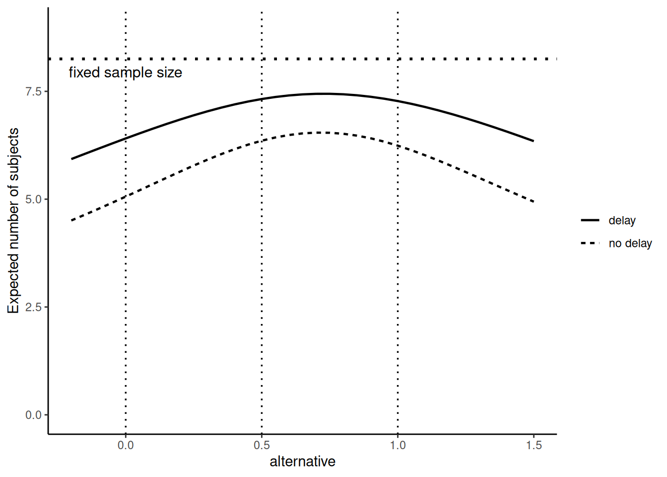
Note that, in contrast, the rejection probabilities are very similar for the different designs:
reject <- c(
    getPowerMeans(gsdWithDelay,
        groups = 1, normalApproximation = TRUE, alternative = deltaRange,
        maxNumberOfSubjects = nMax
    )$overallReject,
    getPowerMeans(gsdWithoutDelay,
        groups = 1, normalApproximation = TRUE, alternative = deltaRange,
        maxNumberOfSubjects = nMax
    )$overallReject
)
dat$reject <- reject

ggplot(data = dat, aes(x = delta, y = reject, group = delay, linetype = factor(delay))) +
    geom_line(size = 0.8) +
    ylim(0, 1) +
    myTheme +
    theme_classic() +
    xlab("alternative") +
    ylab("rejection probability") +
    geom_hline(size = 1, yintercept = 1 - gsdWithDelay$beta, linetype = "dotted") +
    geom_vline(size = 0.6, xintercept = 0, linetype = "dotted") +
    geom_vline(size = 0.6, xintercept = 0.5, linetype = "dotted") +
    geom_vline(size = 0.6, xintercept = 1, linetype = "dotted") +
    labs(linetype = "")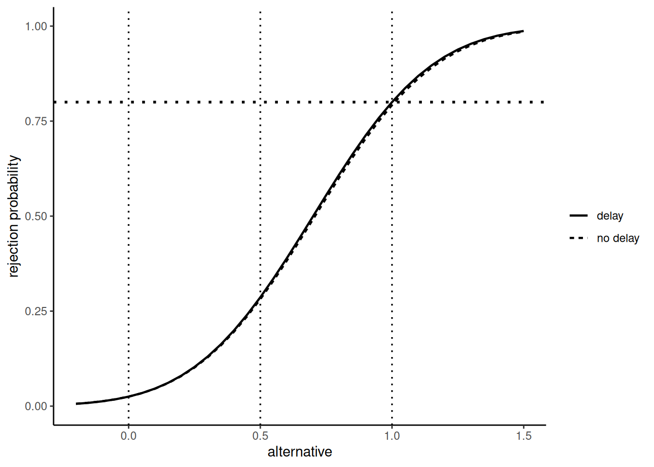
Since we used the maximum sample size nMax from the design with delayed responses, the power is 80% for this design (for the design without delayed response it is slightly lower).
We illustrate the calculation of power and average sample size with an example provided by Schüürhuis (2022), p.68: Suppose it is planned to conduct a parallel group trial with \(N = 175\) subjects per arm to be linearly recruited within \(24\) months in presence of a delay of \(\Delta_t = 5\). The significance level is \(\alpha = 0.025\), the nominal type II error is \(\beta= 0.2\) at a treatment effect of \(\delta = 0.3\). The boundaries are chosen to be calculated using O’Brien-Fleming-like \(\alpha\)- and \(\beta\)-spending functions and the interim is planned after \(I_1 = 0.3\) information has been fully collected. Note that due to the delay, this occurs at \(t_1 = 0.3\cdot 24 + 5 = 12.2\) months. Based on the test statistic available at this point (denoted \(Z_1\) above), it is decided whether or not to stop recruitment. In case the recruitment is stopped, the pipeline data are awaited and the interim analysis then takes place at \(\tilde{t}_1 = 12.2 +5 =17.2\) months. Consequently, the efficacy decision in the interim analysis (if recruitment was stopped) will be performed based on the test statistic \(\tilde{Z}_1\) with an information fraction of \(\tilde{I}_1 = 0.3 + 5/24 = 0.508\). If, on the other hand, recruitment was not stopped at the interim analysis, the second stage is performed and the final analysis takes place at \(24+5=29\) months.
The numbers provided in Table 5.2 of Schüürhuis (2022) for the Hampson and Jennison approach can be obtained with the following commands:
gsdTwoStagesWithDelay <- getDesignGroupSequential(
    kMax = 2,
    alpha = 0.025,
    beta = 0.2,
    typeOfDesign = "asOF",
    typeBetaSpending = "bsOF",
    informationRates = c(0.3, 1),
    delayedInformation = 5 / 24,
    bindingFutility = TRUE
)
results <- getPowerMeans(
    design = gsdTwoStagesWithDelay,
    groups = 2,
    normalApproximation = TRUE,
    alternative = 0.3,
    stDev = 1,
    maxNumberOfSubjects = 350
)

# expected number of subjects table 5.2
round(results$expectedNumberOfSubjects / 2, 3)
[1] 172.6# expected trial duration table 5.2
round(results$earlyStop * 17.2 + (1 - results$earlyStop) * 29, 3)[1] 28.671# power table 5.2
round(results$overallReject, 3)[1] 0.798It has to be noted that the time points of analysis are derived under the assumption of a linear recruitment of patients. Otherwise, these calculations need to be adapted for a non-linear case (which is easy to be done).
The Recruitment Pause approach can be obtained with the following commands (without using the delayedInformation parameter). As above, the interim analysis information is fully observed after \(7.2 + 2\cdot 5 = 17.2\) months, whereas the final information is here after \(24 + 2\cdot 5 = 34\) months:
gsdTwoStagesWithoutDelay <- getDesignGroupSequential(
    kMax = 2,
    alpha = 0.025,
    beta = 0.2,
    typeOfDesign = "asOF",
    typeBetaSpending = "bsOF",
    informationRates = c(0.3 + 5 / 24, 1),
    bindingFutility = FALSE
)

results <- getPowerMeans(
    design = gsdTwoStagesWithoutDelay,
    groups = 2,
    normalApproximation = TRUE,
    alternative = 0.3,
    stDev = 1,
    maxNumberOfSubjects = 350
)

# expected number of subjects table 5.2
round(results$expectedNumberOfSubjects / 2, 3)
[1] 153.053# expected trial duration table 5.2
round(results$earlyStop * 17.2 + (1 - results$earlyStop) * 34, 3)[1] 29.715# power table 5.2
round(results$overallReject, 3)[1] 0.779Plotting designs
The decision boundaries of the delayed response group sequential design can be illustrated as type = 1 plot for the design. This adds the decision boundaries as crosses together with the continuation region. Note that other plot types are directly accounting for the delayed response situation as the required numbers are calculated for this case.
gsdWithDelay |> plot()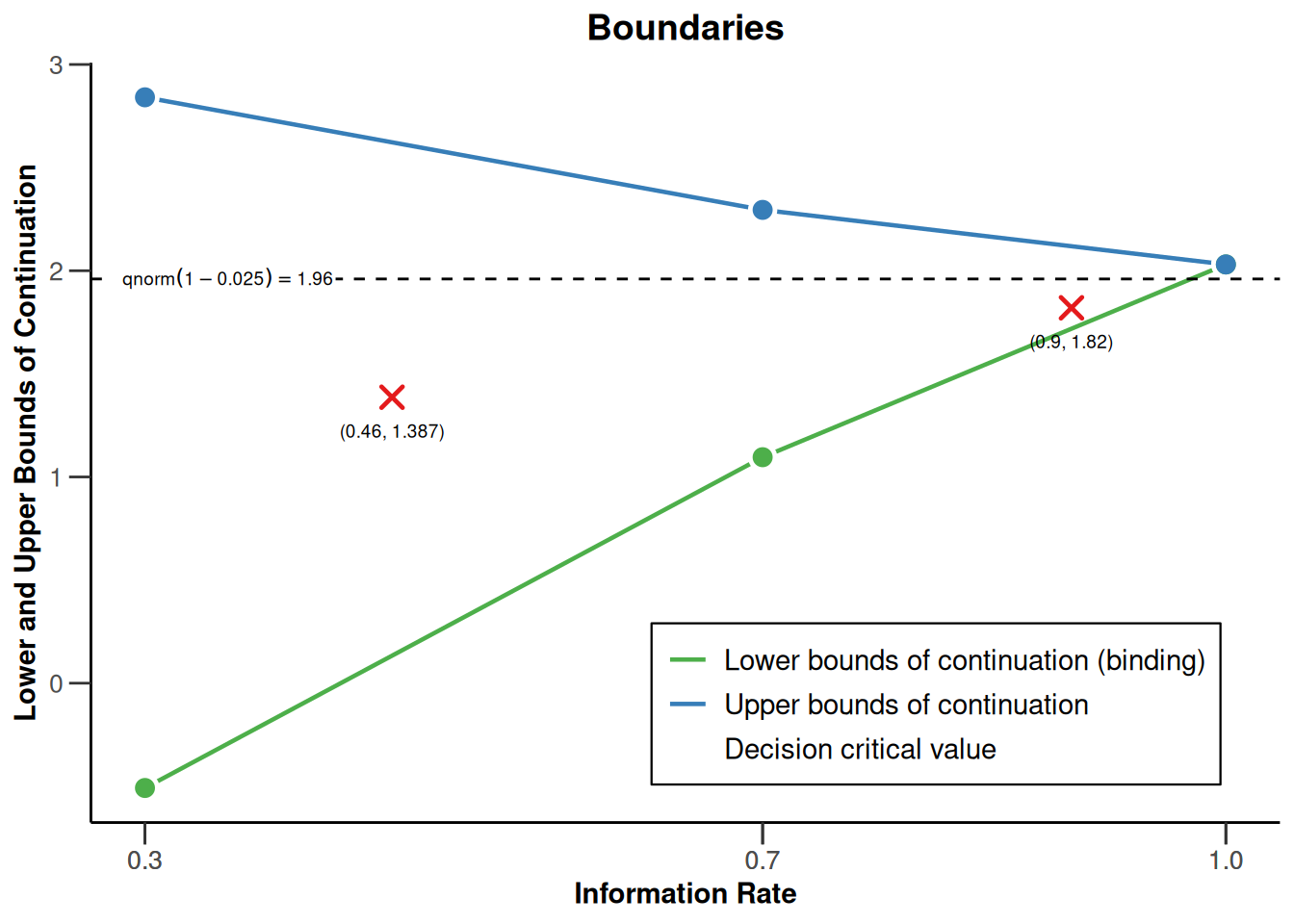
An alternative approach
The approach described so far uses the identity of reversal probabilities to derive the decision boundaries. An alternative approach is to demand two conditions for rejecting the null at a given stage of the trial and spend a specified amount of significance at this stage. This definition is independent of the specification of futility boundaries but can be used with these as well. We show how the (new) rpact function getGroupSequentialProbabilities() can handle this situation.
The definition
At stage \(k\), in order to reject \(H_0\), the test statistic \(Z_k\) needs to exceed the upper continuation bound \(u_k\) and \(\tilde Z_k\) needs to exceed the critical value \(c_k\). Hence, the set of upper continuation boundaries and critical values is defined through the conditions
\[\begin{align}\label{fs:delayedResponseCondition3} \begin{split} &P_{H_0}(Z_1 \geq u_1, \tilde{Z}_k \geq c_1) = \alpha(t_1)\\ &P_{H_0}(Z_1 < u_1, \dots, Z_{k-1} < u_{k-1}, Z_k \geq u_k, \tilde{Z}_k \geq c_k) = \alpha(t_k) - \alpha(t_{k-1}), k = 2, \ldots K - 1, \\ &P_{H_0}(Z_1 < u_1, \dots, Z_{K-1} < u_{K-1}, Z_K \geq u_K) = \alpha(t_K) - \alpha(t_{K-1})\;. \end{split} \end{align}\]
Since this cannot be solved without additional constraints, the critical values \(c_k\) are fixed as \(c_k = \Phi^{-1}(1 - \alpha)\). This makes sense since it often turns out that the optimum boundaries using the reversal probabilities approach are smaller than \(\Phi^{-1}(1 - \alpha)\) and the unadjusted boundary is a reasonable choice for a minimum requirement for rejecting \(H_0\).
Starting by \(k = 1\), the values \(u_k\), \(k = 1,\ldots,K\) with fixed \(c_k\), are successively determined via a root-search.
The conditions for the Type II error rate are the following:
\[\begin{align}\label{fs:delayedResponseCondition4} \begin{split} P_{\delta}(Z_1 \leq &u^0_1) + P_{\delta}(Z_1 \geq u_1, \tilde{Z}_1 \leq c_1) = \beta(t_1)\\ P_{\delta}(Z_1 \in &(u^0_1, u_1), \dots , Z_{k-1} \in (u^0_{k-1}, u_{k-1}), Z_k \leq u^0_k) \\ &+\; P_{\delta}(Z_1 \in (u^0_1, u_1), \dots , Z_{k-1} \in (u^0_{k-1}, u_{k-1}), Z_k \geq u_k , \tilde{Z}_k \leq c_k) = \beta(t_k) - \beta(t_{k-1}), k = 2, \ldots K - 1, \\ P_{\delta}(Z_1 \in &(u^0_1, u_1), \dots , Z_{K-1} \in (u^0_{K-1}, u_{K-1}), Z_K \leq u_K) = \beta(t_K) - \beta(t_{K-1})\;. \end{split} \end{align}\]
The algorithm to derive the acceptance boundaries \(u_1^0, \ldots, u_{K-1}^0\) can be briefly described as follows: At given rejection boundaries \(u_1,\ldots, u_K\) (calculated from above) the algorithm successively calculates the acceptance boundaries using the specifed \(\beta\)-spending function and an arbitrary sample size or “shift” value. If the last stage acceptance critical value is smaller than the last stage critical value, the shift value is increased, otherwise it is decreased. This is repeated until the last stage critical values coincide. The resulting shift value can be interpreted as the maximum necessary sample size to achieve power \(1 - \beta\). Using the algorithm, we have to additionally specify upper and lower boundaries for the shift (which can be interpreted as the maximum sample size for the group sequential design in the prototype case, cf., Wassmer & Brannath, 2016). This is set to be within 0 and 100 which covers practically relevant situations.
Calculation of boundaries
We use the function getGroupSequentialProbabilities() to calculate the critical values by a numerical root search. For this, we define a \(\alpha\)-spending function spend() which can be arbitrarily chosen. Here, we define a function according to the power family of Kim & DeMets with gammaA = 1.345. This value was shown by Hampson & Jennison (2013) to be optimal in a specific context but this does not matter here. The (upper) continuation boundaries \(u_1,\ldots,u_{K -1}\) together with the decision boundaries \(c_1=\cdots = c_{K - 1} = \Phi^{-1}(1 - \alpha) = 1.96\) and the last stage critical boundary \(u_K\) are computed using the uniroot() function as follows.
For \(k = 1\), decisionMatrix is set equal to \[\begin{equation*}
\begin{pmatrix}
u_1 & c_1\\
\infty & \infty
\end{pmatrix}\;,
\end{equation*}\] for \(1 < k < K\), we use \[\begin{equation*}
\begin{pmatrix} -\infty & \ldots &-\infty &u_k & c_k\\ u_1 & \ldots & u_{k-1} & \infty & \infty
\end{pmatrix}\;,
\end{equation*}\] whereas, for \(k = K\), we use \[\begin{equation*}
\begin{pmatrix}
-\infty & \ldots & -\infty &u_K \\
u_1 & \ldots & u_{K-1} & \infty
\end{pmatrix}
\end{equation*}\]
for calculating the stagewise rejection probabilities that yield Type I error rate control with appropriately defined information rates.
###   Derive decision boundaries for delayed response alpha spending approach
alpha <- 0.025
gammaA <- 1.345
tolerance <- 1E-6
#     Specify use function
spend <- function(x, size, gamma) {
    return(size * x^gamma)
}

infRates <- c(28, 54, 96) / 96
kMax <- length(infRates)
delay <- rep(16, kMax - 1) / 96
u <- rep(NA, kMax)
c <- rep(qnorm(1 - alpha), kMax - 1)

for (k in (1:kMax)) {
    if (k < kMax) {
        infRatesPlusDelay <- c(infRates[1:k], infRates[k] + delay[k])
    } else {
        infRatesPlusDelay <- infRates
    }
    u[k] <- uniroot(
        function(x) {
            if (k == 1) {
                d <- matrix(c(
                    x, c[k],
                    Inf, Inf
                ), nrow = 2, byrow = TRUE)
            } else if (k < kMax) {
                d <- matrix(c(
                    rep(-Inf, k - 1), x, c[k],
                    u[1:(k - 1)], Inf, Inf
                ), nrow = 2, byrow = TRUE)
            } else {
                d <- matrix(c(
                    rep(-Inf, k - 1), x,
                    u[1:(k - 1)], Inf
                ), nrow = 2, byrow = TRUE)
            }
            probs <- getGroupSequentialProbabilities(d, infRatesPlusDelay)
            if (k == 1) {
                probs[2, k + 1] - probs[1, k + 1] - spend(infRates[k], alpha, gammaA)
            } else if (k < kMax) {
                probs[2, k + 1] - probs[1, k + 1] - (spend(infRates[k], alpha, gammaA) -
                    spend(infRates[k - 1], alpha, gammaA))
            } else {
                probs[2, k] - probs[1, k] - (spend(infRates[k], alpha, gammaA) -
                    spend(infRates[k - 1], alpha, gammaA))
            }
        },
        lower = -8, upper = 8
    )$root
}
round(u, 5)
[1] 2.43743 2.24413 2.06854We note that any other spending function can be used to define the design. That is, you can also use the spending probabilities of, say, an O`Brien & Fleming design approach that is defined through the shape of the boundaries. Furthermore, it is also possible to use the boundaries \(u_1, \ldots, u_K\) together with the unadjusted critical values \(c_1,\ldots, c_{K - 1}\) in an inverse normal \(p\)-value combination test where the weights are fixed through the planned information rates and the delay.
Calculation of test characteristics
The calculation of the test characteristics is straightforward and can be derived for designs with or without futility boundaries. In the following example, we show how to derive lower continuation (or futility) boundaries \(u^0_1, \ldots,u^0_{K -1 }\) that are based on a \(\beta\)-spending function approach. As above, we use the same Kim & DeMets spending function with gammaB = 1.345. Due to numerical reasons, we do not use the uniroot() function here but a bisection method to numerically search for the boundaries.
beta <- 0.1
gammaB <- 1.345
u0 <- rep(NA, kMax)
cLower1 <- 0
cUpper1 <- 100
prec1 <- 1
iteration <- 1E5
while (prec1 > tolerance) {
    shift <- (cLower1 + cUpper1) / 2
    for (k in (1:kMax)) {
        if (k < kMax) {
            infRatesPlusDelay <- c(infRates[1:k], infRates[k] + delay[k])
        } else {
            infRatesPlusDelay <- infRates
        }
        nz <- matrix(rep(sqrt(infRatesPlusDelay), 2), nrow = 2, byrow = TRUE) * sqrt(shift)
        prec2 <- 1
        cLower2 <- -8
        cUpper2 <- 8
        while (prec2 > tolerance) {
            x <- (cLower2 + cUpper2) / 2
            if (k == 1) {
                d2 <- matrix(c(
                    u[k], c[k],
                    Inf, Inf
                ), nrow = 2, byrow = TRUE) - nz
                probs <- getGroupSequentialProbabilities(d2, infRatesPlusDelay)
                ifelse(pnorm(x - nz[1]) + probs[1, k + 1] < spend(infRates[k], beta, gammaB),
                    cLower2 <- x, cUpper2 <- x
                )
            } else if (k < kMax) {
                d1 <- matrix(c(
                    pmin(u0[1:(k - 1)], u[1:(k - 1)]), x,
                    u[1:(k - 1)], Inf
                ), nrow = 2, byrow = TRUE) - nz[, 1:k]
                probs1 <- getGroupSequentialProbabilities(d1, infRatesPlusDelay[1:k])
                d2 <- matrix(c(
                    pmin(u0[1:(k - 1)], u[1:(k - 1)]), u[k], c[k],
                    u[1:(k - 1)], Inf, Inf
                ), nrow = 2, byrow = TRUE) - nz
                probs2 <- getGroupSequentialProbabilities(d2, infRatesPlusDelay)
                ifelse(probs1[1, k] + probs2[1, k + 1] < spend(infRates[k], beta, gammaB) -
                    spend(
                        infRates[k - 1],
                        beta, gammaB
                    ),
                cLower2 <- x, cUpper2 <- x
                )
            } else {
                d1 <- matrix(c(
                    pmin(u0[1:(k - 1)], u[1:(k - 1)]), x,
                    u[1:(k - 1)], Inf
                ), nrow = 2, byrow = TRUE) - nz
                probs <- getGroupSequentialProbabilities(d1, infRates)
                ifelse(probs[1, k] < spend(infRates[k], beta, gammaB) -
                    spend(infRates[k - 1], beta, gammaB),
                cLower2 <- x, cUpper2 <- x
                )
            }
            iteration <- iteration - 1
            ifelse(iteration > 0, prec2 <- cUpper2 - cLower2, prec2 <- 0)
        }
        u0[k] <- x
    }
    ifelse(u0[kMax] < u[kMax], cLower1 <- shift, cUpper1 <- shift)
    ifelse(iteration > 0, prec1 <- cUpper1 - cLower1, prec1 <- 0)
}
round(u0, 5)
[1] -0.40891 0.66367 2.06854round(shift, 2)[1] 12round(shift / (qnorm(1 - alpha) + qnorm(1 - beta))^2, 3)[1] 1.142We can compare these values with the “original” \(\beta\)-spending approach with non-binding futility boundaries using the function getDesignGroupSequential():
x <- getDesignGroupSequential(
    informationRates = infRates,
    typeOfDesign = "asKD",
    typeBetaSpending = "bsKD",
    gammaA = gammaA,
    gammaB = gammaB,
    alpha = alpha,
    beta = beta,
    bindingFutility = FALSE
)
round(x$futilityBounds, 5)
[1] -0.19958 0.80463round(x$criticalValues, 5)[1] 2.59231 2.39219 2.10214round(getDesignCharacteristics(x)$inflationFactor, 3)[1] 1.146Conclusions
We have shown how to handle a group sequential design with delayed responses in two diffenrent ways. So far, we have implemented the approach proposed by Hampson & Jennison (2013) that is based on reversal probabilities. The direct usage of the delayed information within the design definition make it easy for the user to apply these designs to commonly used trials with continuous, binary, and time to event endpoints. We have also shown how to use the getGroupSequentialProbabilities() function to derive the critical values and the test characteristics for the alternative approach that “more directly” determines the critical values through a spending function approach.
System: rpact 4.4.0.9305, R version 4.6.0 (2026-04-24), platform: x86_64-pc-linux-gnu
To cite R in publications use:
R Core Team (2026). R: A Language and Environment for Statistical Computing. R Foundation for Statistical Computing, Vienna, Austria. doi:10.32614/R.manuals https://doi.org/10.32614/R.manuals. https://www.R-project.org/.
To cite package ‘rpact’ in publications use:
Wassmer G, Pahlke F (2026). rpact: Confirmatory Adaptive Clinical Trial Design and Analysis. R package version 4.4.0.9305. doi:10.32614/CRAN.package.rpact
Wassmer G, Brannath W (2025). Group Sequential and Confirmatory Adaptive Designs in Clinical Trials, 2nd edition. Springer, Cham, Switzerland. ISBN 978-3-031-89668-2. doi:10.1007/978-3-031-89669-9 https://doi.org/10.1007/978-3-031-89669-9.