getSampleSizeCounts(
    design = NULL,
    ...,
    lambda1 = NA_real_,
    lambda2 = NA_real_,
    lambda = NA_real_,
    theta = NA_real_,
    thetaH0 = 1,
    overdispersion = 0,
    fixedExposureTime = NA_real_,
    accrualTime = NA_real_,
    accrualIntensity = NA_real_,
    followUpTime = NA_real_,
    maxNumberOfSubjects = NA_real_,
    allocationRatioPlanned = NA_real_
)Count Data with rpact
Planning
Count Data
Rates
This document describes how sample size and power calculations for count data can be performed using rpact. This is shown for the fixed sample and the group sequential case, thereby illustrating different ways of entering recruitment and observation schemes. It also describes how blinded sample size recalculation procedures can be performed.
Introduction
Examples for count data described in the literature are
- exacerbations in asthma and chronic obstructive pulmonary disease (COPD)
- counts of brain lesions by MRI in Multiple Sclerosis (MS)
- relapses in pediatric MS
- hospitalizations in heart failure trials
- number of occurrences of adverse events
Typically, the count outcome is assumed to be distributed according to a negative binomial distribution and the hypothesis to be tested is
\[ H_0 : \theta = \frac{\lambda_1}{\lambda_2} = \delta_0\;, \]
where \(\lambda_i\) are the mean rates (in one time unit) of a negative binomial distributed random variable \(Y_{ijk}\) with overdispersion (shape) parameter \(\phi\),
\[ Y_{ijk} \sim NB(t_{ijk}\,\lambda_i, \phi)\, , \]
where \(t_{ijk}\) refers to the exposure time of subject \(j\) in treatment group \(i\) at interim stage \(k\) of the group sequential test procedure (cf., Mütze et al., 2019). The expectation and variance of \(Y_{ijk}\) are given by
\[ E(Y_{ijk}) = t_{ijk}\lambda_i \quad \text{ and }\quad Var(Y_{ijk}) = t_{ijk}\lambda_i + \phi(t_{ijk}\lambda_i)^2, \]
respectively, i.e., the case \(\phi = 0\) refers to the case where \(Y_{ijk}\) is Poisson distributed. For the fixed sample case, the index \(k\) for the interim stage is omitted. In superiority trials, \(\delta_0 = 1\), whereas, for non-inferiority trials, a positive non-inferiority margin \(\delta_0\) is specified.
In many cases, each subject is observed a given length of time, e.g., one year. In this case, \(t_{ijk} \equiv t\), and, as will be shown below, the sample size formulas described in the literature are applicable. If subjects entering the study have different exposure times, typically an accrual time is followed by an additional follow-up time. If subjects enter the study in an accrual period \([0;\, a]\) and the study time is \(t_{max}\), at time point \(t_k\), the time under exposure for subject \(j\) in treatment \(i\) at stage \(k\) of the trial is \(t_{ijk} = t_{k} - a_{ij}\) with \(t_K = t_{max}\) and \(a_{ij}\) denoting the recruitment time for subject \(j\) in treatment \(i\). This more general approach is specifically necessary if the observation times at interim stages need to be estimated. This will also be illustrated by examples later on.
For group sequential designs, the test statistic is based on the Wald statistic, which is the difference of the rates on the log-scale divided by its standard error. As shown in Mütze et al. (2019), if Maximum Likelihood estimates are used to estimate the true parameters, the sequence of Wald statistics asymptotically has the independent and normally distributed increments property. For designs with interim stages, it is essential that interim analyses take place after specified amounts of information. The information level of the Wald statistic (the Fisher information) at stage \(k\) is given by
\[ {\cal I}_k = \left(\frac{1}{ \sum_{j = 1}^{n_1} \frac{t_{1jk}\lambda_1}{1 + \phi\,t_{1jk}\lambda_1}} + \frac{1}{ \sum_{j = 1}^{n_2}\frac{t_{2jk}\lambda_2}{1 + \phi\,t_{2jk}\lambda_2}}\right)^{-1}\;, \] which simplifies to
\[ {\cal I} = n_2\;\left(\frac{1}{t} (\frac{1}{\lambda_2} + \frac{1}{r\,\lambda_1}) + \phi\,(1 + \frac{1}{r})\right)^{-1} \;, \]
if \(t_{ijk} \equiv t\), i.e., if all subjects have complete observations. From these terms, essentially, the sample size and other calculations for a count data type design are derived.
The sample size calculation to meet power \(1-\beta\) for two-sample comparisons is performed for
- for group sequential designs, the type of design (e.g., \(\alpha\)-spending),
- an assumed \(\lambda_1\) and \(\lambda_2\),
- assumed exposure times \(t_{ijk}\) for treatment \(i\), and subjects \(j = 1,\ldots,n_i\), at interim stage \(k\),
- a planned allocation ratio \(r = n_1/n_2\),
- and an assumed overdispersion \(\phi \geq 0\).
rpact Functions for Count Data
getSampleSizeCounts() performs sample size calculations for count data designs. You can specify
- a group sequential or a fixed sample size setting
- either \(\lambda_1\) and \(\lambda_2\), or \(\lambda_2\) and \(\theta\), or the pooled \(\lambda\) and \(\theta\), the latter being essential for blinded sample size reassessment (SSR) procedures (see below). \(\lambda_1\) and \(\theta\) can be vectors
- different ways of calculation: fixed exposure time, accrual and study time, or accrual and fixed number of subjects
- staggered subjects entry
The usage of the function (listing the parameters that can be specified) is as follows:
which will now be illustrated by examples.
getPowerCounts() conversely calculates the power at given sample sizes, and essentially the same parameters can be specified.
Fixed Sample Size Designs and Blinded Sample Size Reassessment
Fixed exposure time
Consider the clinical trial in COPD subjects from Zhu and Lakkis (2014). Assume that a new therapy is assumed to decrease the exacerbation rate from 0.80 to 0.68 (15% decrease relative to control) within an observation period of 0.75 years, i.e., each subject has a equal follow-up of 0.75 years. Subjects are randomly allocated to treatment and control with equal allocation 1:1.
The sample size that yields 80% power for detecting such a difference, if the overdispersion is assumed to be equal to 0.4, is obtained as follows.
First, load the rpact package
library(rpact)
packageVersion("rpact") # version should be version 3.5.0 or higher
[1] '4.4.0.9305'The planned sample sizes are achieved by the following code:
example1 <- getSampleSizeCounts(
    alpha = 0.025,
    beta = 0.2,
    lambda2 = 0.8,
    theta = 0.85,
    overdispersion = 0.4,
    fixedExposureTime = 0.75
)
The example1$nFixed1 element is the number of subjects in the treatment group, example1$nFixed2 refers to the number of subjects in the control group:
c(example1$nFixed1, example1$nFixed2)[1] 1316 1316and we conclude that N = 2632 subjects in total are needed to provide 80% power.
Conversely, getPowerCounts() performs the power calculation at given sample size, and note directionUpper = FALSE to specify that the power is directed for \(\theta < 1\):
example2 <- getPowerCounts(
    alpha = 0.025,
    lambda2 = 0.8,
    theta = 0.85,
    overdispersion = 0.4,
    fixedExposureTime = 0.75,
    directionUpper = FALSE,
    maxNumberOfSubjects = example1$nFixed
)
example2$overallReject
[1] 0.8000924The following graph illustrates the sample sizes for stronger effects \(\theta\). Note that for this plot only the lower and upper bound of \(\theta\) need to be specified:
getSampleSizeCounts(
    alpha = 0.025,
    beta = 0.2,
    lambda2 = 0.8,
    theta = c(0.75, 0.85),
    overdispersion = 0.4,
    fixedExposureTime = 0.75
) |>
    plot()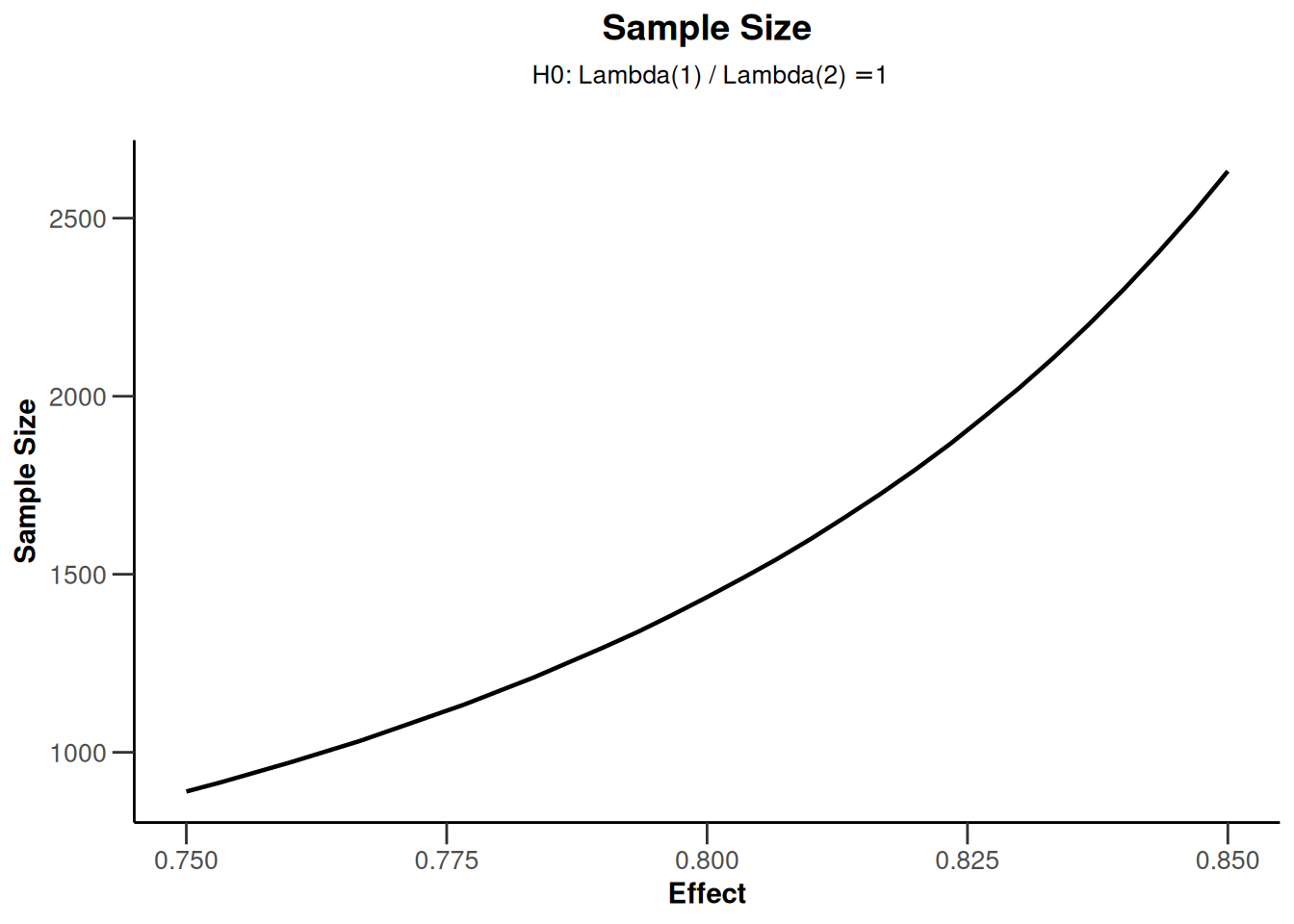
In the fixed sample case this is the only available plot type (type = 5).
For getPowerCounts(), the only available plot type in the fixed sample case is type = 7. The following graph also illustrates how elements can be added to the ggplot2 object:
getPowerCounts(
    alpha = 0.025,
    lambda2 = 0.8,
    theta = c(0.8, 1),
    overdispersion = 0.4,
    fixedExposureTime = 0.75,
    directionUpper = FALSE,
    maxNumberOfSubjects = example1$nFixed
) |>
    plot(markdown = FALSE) +
    ylab("Power") +
    ggtitle("Power for count data design for varying effect") +
    geom_hline(linewidth = 0.5, yintercept = 0.025, linetype = "dotted") +
    geom_hline(linewidth = 0.5, yintercept = 0.8, linetype = "dotted")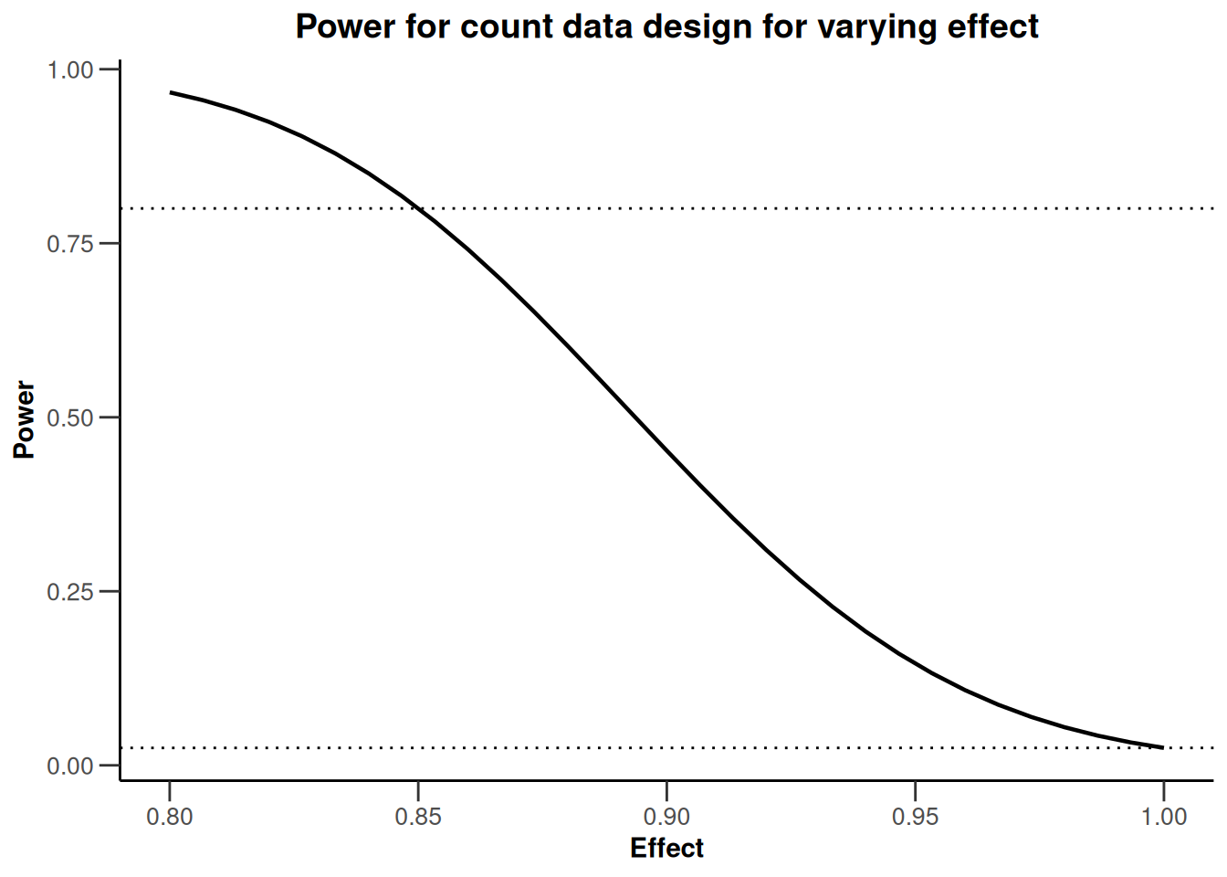
The influence of the overdispersion parameter \(\phi \geq 0\) on the total sample size is illustrated in the following graph for increasing effect \(\theta\):
results <- c()
for (theta in seq(0.75, 0.85, 0.05)) {
    for (phi in seq(0, 1, 0.1)) {
        results <- rbind(
            results,
            getSampleSizeCounts(
                alpha = 0.025,
                beta = 0.2,
                lambda2 = 0.8,
                theta = theta,
                overdispersion = phi,
                fixedExposureTime = 0.75
            ) |>
                as.data.frame()
        )
    }
}
ggplot(
    data = results,
    aes(x = overdispersion, y = nFixed, group = theta, color = as.factor(theta))
) +
    xlab("Overdispersion") +
    ylab("Total sample size") +
    geom_line(linewidth = 1.1) +
    geom_hline(linewidth = 0.5, yintercept = 1000, linetype = "dotted") +
    geom_hline(linewidth = 0.5, yintercept = 2000, linetype = "dotted") +
    geom_hline(linewidth = 0.5, yintercept = 3000, linetype = "dotted") +
    labs(color = "Theta") +
    theme_classic()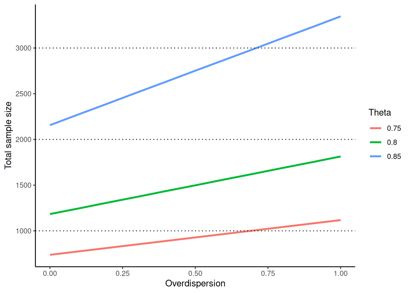
Zhu and Lakkis (2014) proposed three methods for calculating the sample size and the methodology implemented in rpact refers to the M2 method described in their paper. The M2 method corresponds to the sample size formulas given in, e.g., Friede and Schmidli (2010a, 2010b) and Mütze et al (2019). It is in fact easy to recalculate the sample sizes in Table 1 of their paper:
results <- c()
for (phi in c(0.4, 0.7, 1, 1.5)) {
    for (theta in c(0.85, 1.15)) {
        for (lambda2 in seq(0.8, 1.4, 0.2)) {
            results <- c(results, getSampleSizeCounts(
                alpha = 0.025,
                beta = 0.2,
                lambda2 = lambda2,
                theta = theta,
                overdispersion = phi,
                fixedExposureTime = 0.75
            )$nFixed1)
        }
    }
}
cat(paste0(results, collapse = ", "))
1316, 1101, 957, 854, 1574, 1324, 1157, 1037, 1494, 1279, 1135, 1033, 1815, 1565, 1398, 1278, 1673, 1457, 1313, 1211, 2056, 1806, 1639, 1520, 1970, 1754, 1611, 1508, 2458, 2208, 2041, 1921
Similarly, Table 2 results (column M2) with varying allocation between the treatment arms can be reconstructed by
results <- c()
for (phi in c(1, 5)) {
    for (theta in c(0.5, 1.5)) {
        for (lambda2 in c(2, 5, 10)) {
            for (r in c(2 / 3, 1, 3 / 2)) {
                results <- c(results, getSampleSizeCounts(
                    alpha = 0.025,
                    beta = 0.2,
                    lambda2 = lambda2,
                    theta = theta,
                    overdispersion = phi,
                    allocationRatioPlanned = r,
                    fixedExposureTime = 1
                )$nFixed)
            }
        }
    }
}
cat(paste0(results, collapse = ", "))
124, 116, 117, 90, 86, 88, 80, 76, 79, 280, 272, 287, 232, 224, 235, 215, 208, 217, 395, 376, 389, 363, 348, 360, 352, 338, 350, 1075, 1036, 1082, 1027, 988, 1030, 1012, 972, 1013
Slight deviations resulting from rounding errors.
Optimum allocation ratio
With the getSampleSizeCounts() function, it is easy to determine the allocation ratio that provides the smallest overall sample size at given power \(1 - \beta\). This can be done by setting allocationRatioPlanned = 0. In the example from above,
example3 <- getSampleSizeCounts(
    alpha = 0.025,
    beta = 0.2,
    lambda2 = 0.8,
    theta = 0.85,
    overdispersion = 0.4,
    allocationRatioPlanned = 0,
    fixedExposureTime = 0.75
)example3$allocationRatioPlanned[1] 1.068791example3$nFixed[1] 2629calculates the optimum allocation ratio to be equal to 1.069, thereby reducing the necessary sample size only very slightly from 2632 to 2629. With this result, it might not be reasonable at all to deviate from a planned 1:1 allocation.
Usage in blinded sample size reestimation (SSR)
Friede and Schmidli (2010a, 2010b) consider blinded SSR procedures with count data. They show that blinded SSR to reestimate the overdispersion parameter maintains the required power without increasing the Type I error rate. The procedure is simply to calculate the overdispersion at interim in a blinded manner and to recalculate the sample size with a pooled event rate estimate and under the assumption of the originally assumed effect.
For example, if in the situation from above, the overdispersion was estimated from the pooled sample to be, say, 0.352, and the overall event rate is estimated as \(\hat\lambda = 0.921\), the recalculated sample size is
example4 <- getSampleSizeCounts(
    alpha = 0.025,
    beta = 0.2,
    lambda = 0.921,
    theta = 0.85,
    overdispersion = 0.352,
    fixedExposureTime = 0.75
)
example4$nFixed
[1] 2152thus reducing the necessary sample size from 2632 to 2152. Note that, of course, it is important when the interim review is performed. If it is done early, the nuisance parameters \(\lambda\) and \(\phi\) cannot be estimated with sufficient precision, if it is done very late, the recalculated sample size might be smaller than the already obtained sample size. This of course also has an impact on the test characteristics and might be investigated by simulations (Friede and Schmidli, 2010a). Methods for blinded estimation are compared by Schneider et al. (2013).
For checking the results of rpact, the sample sizes in Table 1 from Friede and Schmidli (2010b) can be reconstructed by
results <- c()
for (theta in c(0.7, 0.8)) {
    for (phi in c(0.4, 0.5, 0.6)) {
        for (lambda in c(1, 1.5, 2)) {
            results <- c(results, getSampleSizeCounts(
                alpha = 0.025,
                beta = 0.2,
                lambda = lambda,
                theta = theta,
                overdispersion = phi,
                fixedExposureTime = 1
            )$nFixed2)
        }
    }
}
cat(paste0(results, collapse = ", "))
177, 135, 114, 190, 147, 126, 202, 159, 138, 446, 339, 286, 477, 371, 318, 509, 402, 349
and
results <- c()
for (theta in c(0.7, 0.8)) {
    for (phi in c(0.4, 0.5, 0.6)) {
        for (lambda in c(1, 1.5, 2)) {
            results <- c(results, getSampleSizeCounts(
                alpha = 0.025,
                beta = 0.1,
                lambda = lambda,
                theta = theta,
                overdispersion = phi,
                fixedExposureTime = 1
            )$nFixed2)
        }
    }
}
cat(paste0(results, collapse = ", "))
237, 180, 152, 254, 197, 168, 270, 213, 185, 597, 454, 383, 639, 496, 425, 681, 539, 467
Slight deviations resulting from rounding errors.
The non-inferiority case
For the non-inferiority case, a non-inferiority margin \(\delta_0\) needs to be specified and entered as thetaH0. Typically, as the planning alternative, no difference in the event rates is assumed between the treatment groups (i.e., \(\theta = 1\)). In that case, the control arm sample sizes from Table 2 and Table 3 from Friede and Schmidli (2010b) are obtained with
results <- c()
for (delta0 in c(1.15, 1.2)) {
    for (phi in c(0.4, 0.5, 0.6)) {
        for (lambda in c(1, 1.5, 2)) {
            results <- c(results, getSampleSizeCounts(
                alpha = 0.025,
                beta = 0.2,
                lambda = lambda,
                theta = 1,
                thetaH0 = delta0,
                overdispersion = phi,
                fixedExposureTime = 1
            )$nFixed2)
        }
    }
}
cat(paste0(results, collapse = ", "))
1126, 858, 724, 1206, 938, 804, 1286, 1018, 885, 662, 504, 426, 709, 551, 473, 756, 599, 520
Designs with Interim Stages
We will now consider count data designs with interim stages. First, you need to specify the design which is here defined as an O’Brien and Fleming alpha spending function design with interim analyses planned after 40% and 70% of the information:
design <- getDesignGroupSequential(
    informationRates = c(0.4, 0.7, 1),
    typeOfDesign = "asOF"
)
Fixed exposure time
Suppose study subjects are observed with fixed exposure time of 12 months and have event rates 0.2 and 0.3 in the treatment and the control arm, respectively, with an overdispersion parameter equal to 1. Specify these parameters as follows to obtain the summary:
getSampleSizeCounts(
    design = design,
    lambda1 = 0.2,
    lambda2 = 0.3,
    fixedExposureTime = 12,
    overdispersion = 1.5
) |>
    summary()
Sample size calculation for a count data endpoint
Sequential analysis with a maximum of 3 looks (group sequential design), one-sided overall significance level 2.5%, power 80%. The results were calculated for a two-sample Wald-test for count data, H0: lambda(1) / lambda(2) = 1, H1: effect = 0.667, lambda(1) = 0.2, lambda(2) = 0.3, overdispersion = 1.5, fixed exposure time = 12.
| Stage | 1 | 2 | 3 |
|---|---|---|---|
| Planned information rate | 40% | 70% | 100% |
| Cumulative alpha spent | 0.0004 | 0.0074 | 0.0250 |
| Stage levels (one-sided) | 0.0004 | 0.0073 | 0.0227 |
| Efficacy boundary (z-value scale) | 3.357 | 2.445 | 2.001 |
| Efficacy boundary (t) | 0.459 | 0.658 | 0.752 |
| Cumulative power | 0.0580 | 0.4682 | 0.8000 |
| Maximum number of subjects | 360.0 | ||
| Information over stages | 19.4 | 33.9 | 48.5 |
| Expected information under H0 | 48.4 | ||
| Expected information under H0/H1 | 46.9 | ||
| Expected information under H1 | 40.8 | ||
| Exit probability for efficacy (under H0) | 0.0004 | 0.0070 | |
| Exit probability for efficacy (under H1) | 0.0580 | 0.4102 |
Legend:
- (t): treatment effect scale
This summary displays the maximum amount of information (round(example5$maxInformation, 2) = 48.47) that needs to be achieved with N = 360 subjects together with stopping probabilities under \(H_0\), midway between \(H_0\) and \(H_1\), under \(H_1\), and stopping probabilities under \(H_0\) and \(H_1\) if interim analyses are performed at \({\cal I}_1 =\) 19.39 and \({\cal I}_2 =\) 33.93, and the final analysis at \({\cal I}_3 =\) 48.47.
If non-binding futility stops are planned, these might be derived from an O’Brien and Fleming beta spending function with \(\beta = 0.2\), i.e., the following design as displayed in the graph below:
designFutility <- getDesignGroupSequential(
    informationRates = c(0.4, 0.7, 1),
    beta = 0.2,
    typeOfDesign = "asOF",
    typeBetaSpending = "bsOF",
    bindingFutility = FALSE
)
designFutility |>
    plot()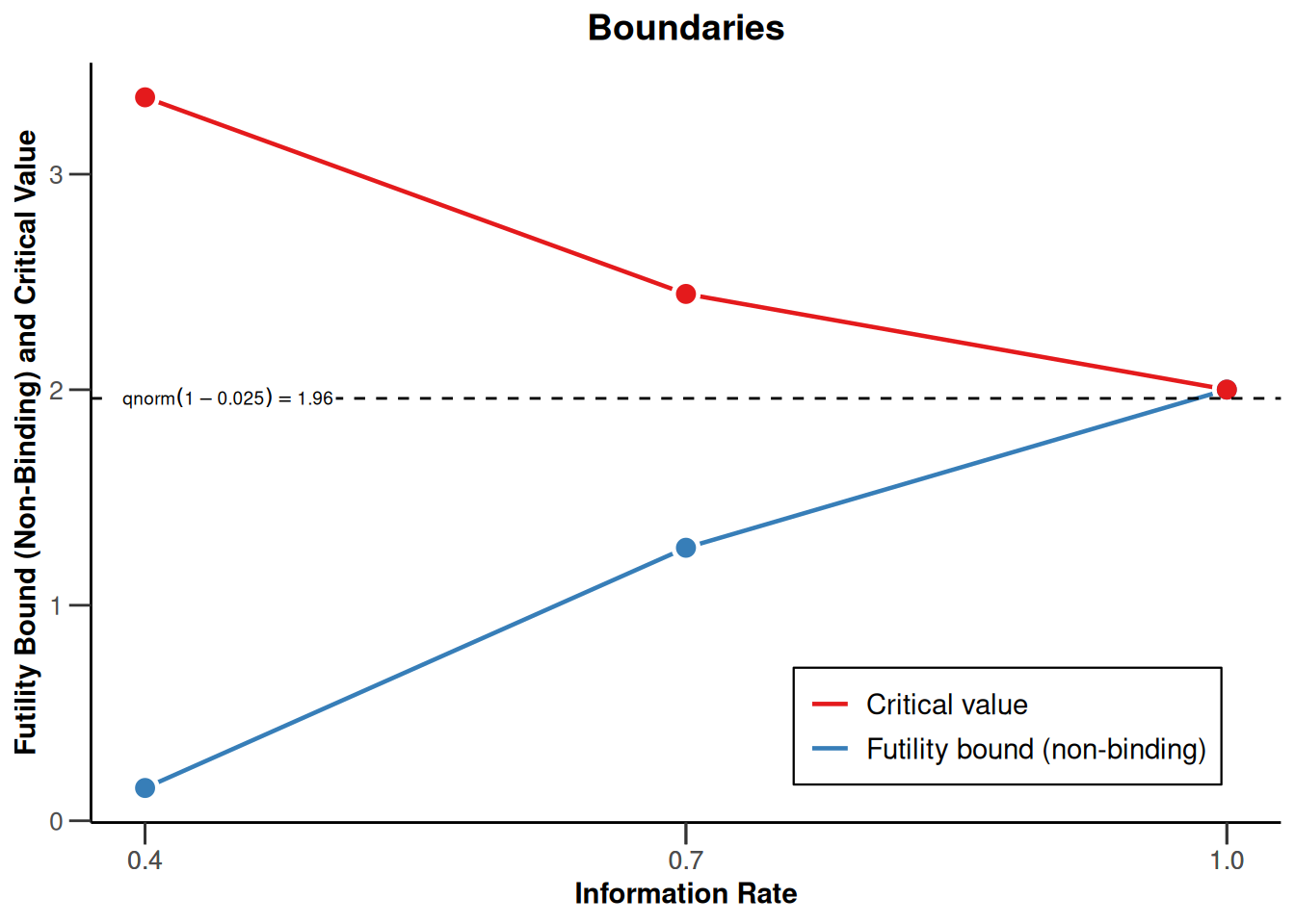
This yields the following test characteristics with additional futility stop probabilities, resulting in a slightly higher number of subjects and increased information levels necessary to achieve power 80%:
getSampleSizeCounts(
    design = designFutility,
    lambda1 = 0.2,
    lambda2 = 0.3,
    fixedExposureTime = 12,
    overdispersion = 1.5
) |>
    summary()
Sample size calculation for a count data endpoint
Sequential analysis with a maximum of 3 looks (group sequential design), one-sided overall significance level 2.5%, power 80%. The results were calculated for a two-sample Wald-test for count data, H0: lambda(1) / lambda(2) = 1, H1: effect = 0.667, lambda(1) = 0.2, lambda(2) = 0.3, overdispersion = 1.5, fixed exposure time = 12.
| Stage | 1 | 2 | 3 |
|---|---|---|---|
| Planned information rate | 40% | 70% | 100% |
| Cumulative alpha spent | 0.0004 | 0.0074 | 0.0250 |
| Cumulative beta spent | 0.0427 | 0.1256 | 0.2000 |
| Stage levels (one-sided) | 0.0004 | 0.0073 | 0.0227 |
| Efficacy boundary (z-value scale) | 3.357 | 2.445 | 2.001 |
| Futility boundary (z-value scale) | 0.152 | 1.267 | |
| Efficacy boundary (t) | 0.476 | 0.670 | 0.762 |
| Futility boundary (t) | 0.968 | 0.814 | |
| Cumulative power | 0.0688 | 0.5133 | 0.8000 |
| Maximum number of subjects | 394.0 | ||
| Information over stages | 21.3 | 37.3 | 53.3 |
| Expected information under H0 | 29.8 | ||
| Expected information under H0/H1 | 39.4 | ||
| Expected information under H1 | 41.3 | ||
| Overall exit probability (under H0) | 0.5608 | 0.3491 | |
| Overall exit probability (under H1) | 0.1115 | 0.5274 | |
| Exit probability for efficacy (under H0) | 0.0004 | 0.0070 | |
| Exit probability for efficacy (under H1) | 0.0688 | 0.4446 | |
| Exit probability for futility (under H0) | 0.5604 | 0.3421 | |
| Exit probability for futility (under H1) | 0.0427 | 0.0829 |
Legend:
- (t): treatment effect scale
Estimate observation time under uniform recruitment
Similar to survival designs (see, e.g., Planning a Survival Trial with rpact) it is possible with the getSampleSizeCounts() function to calculate calendar times where the information is estimated to be observed under the given parameters.
For the first case, suppose there is uniform recruitment of subjects over 6 months, and subjects are followed for a prespecified time period which is identical for all subjects as above. Specify accrualTime = 6 as an additional function parameter and obtain the following summary:
example7 <- getSampleSizeCounts(
    design = designFutility,
    lambda1 = 0.2,
    lambda2 = 0.3,
    overdispersion = 1.5,
    fixedExposureTime = 12,
    accrualTime = 6
)
example7 |>
    summary()
Sample size calculation for a count data endpoint
Sequential analysis with a maximum of 3 looks (group sequential design), one-sided overall significance level 2.5%, power 80%. The results were calculated for a two-sample Wald-test for count data, H0: lambda(1) / lambda(2) = 1, H1: effect = 0.667, lambda(1) = 0.2, lambda(2) = 0.3, overdispersion = 1.5, fixed exposure time = 12, accrual time = 6.
| Stage | 1 | 2 | 3 |
|---|---|---|---|
| Planned information rate | 40% | 70% | 100% |
| Cumulative alpha spent | 0.0004 | 0.0074 | 0.0250 |
| Cumulative beta spent | 0.0427 | 0.1256 | 0.2000 |
| Stage levels (one-sided) | 0.0004 | 0.0073 | 0.0227 |
| Efficacy boundary (z-value scale) | 3.357 | 2.445 | 2.001 |
| Futility boundary (z-value scale) | 0.152 | 1.267 | |
| Efficacy boundary (t) | 0.429 | 0.670 | 0.762 |
| Futility boundary (t) | 0.964 | 0.814 | |
| Cumulative power | 0.0688 | 0.5133 | 0.8000 |
| Number of subjects | 308.0 | 394.0 | 394.0 |
| Expected number of subjects under H1 | 384.4 | ||
| Calendar time | 4.70 | 7.11 | 18.00 |
| Expected study duration under H1 | 10.77 | ||
| Information over stages | 21.3 | 37.3 | 53.3 |
| Expected information under H0 | 29.8 | ||
| Expected information under H0/H1 | 39.4 | ||
| Expected information under H1 | 41.3 | ||
| Overall exit probability (under H0) | 0.5608 | 0.3491 | |
| Overall exit probability (under H1) | 0.1115 | 0.5274 | |
| Exit probability for efficacy (under H0) | 0.0004 | 0.0070 | |
| Exit probability for efficacy (under H1) | 0.0688 | 0.4446 | |
| Exit probability for futility (under H0) | 0.5604 | 0.3421 | |
| Exit probability for futility (under H1) | 0.0427 | 0.0829 |
Legend:
- (t): treatment effect scale
You might also use the gscounts package in order to obtain very similar results. The relevant functionality for count data, however, is included in rpact and the maintainer of gscounts encourages the use of rpact.
Sample size for variable exposure time with uniform recruitment
A different situation is given if subjects have varying exposure time. For this setting, assume we again have uniform recruitment of subjects over 6 months, but the study ends 12 months after the last subject entered the study. That is, the study is planned to be conducted in 18 months, having subjects that are observed (i.e., under exposure) between 12 and 18 months.
In order to perform the sample size calculation for this case, instead of fixedExposureTime, the parameter followUpTime has to specified. It is the assumed (additional) follow-up time for the study and so the total study duration is accrualTime + followUpTime.
example8 <- getSampleSizeCounts(
    design = designFutility,
    lambda1 = 0.2,
    lambda2 = 0.3,
    overdispersion = 1.5,
    accrualTime = 6,
    followUpTime = 12
)
example8 |>
    summary()
Sample size calculation for a count data endpoint
Sequential analysis with a maximum of 3 looks (group sequential design), one-sided overall significance level 2.5%, power 80%. The results were calculated for a two-sample Wald-test for count data, H0: lambda(1) / lambda(2) = 1, H1: effect = 0.667, lambda(1) = 0.2, lambda(2) = 0.3, overdispersion = 1.5, accrual time = 6, follow-up time = 12.
| Stage | 1 | 2 | 3 |
|---|---|---|---|
| Planned information rate | 40% | 70% | 100% |
| Cumulative alpha spent | 0.0004 | 0.0074 | 0.0250 |
| Cumulative beta spent | 0.0427 | 0.1256 | 0.2000 |
| Stage levels (one-sided) | 0.0004 | 0.0073 | 0.0227 |
| Efficacy boundary (z-value scale) | 3.357 | 2.445 | 2.001 |
| Futility boundary (z-value scale) | 0.152 | 1.267 | |
| Efficacy boundary (t) | 0.437 | 0.670 | 0.762 |
| Futility boundary (t) | 0.964 | 0.814 | |
| Cumulative power | 0.0688 | 0.5133 | 0.8000 |
| Number of subjects | 304.0 | 380.0 | 380.0 |
| Expected number of subjects under H1 | 371.5 | ||
| Calendar time | 4.81 | 7.42 | 18.00 |
| Expected study duration under H1 | 10.95 | ||
| Information over stages | 21.3 | 37.3 | 53.3 |
| Expected information under H0 | 29.8 | ||
| Expected information under H0/H1 | 39.4 | ||
| Expected information under H1 | 41.3 | ||
| Overall exit probability (under H0) | 0.5608 | 0.3491 | |
| Overall exit probability (under H1) | 0.1115 | 0.5274 | |
| Exit probability for efficacy (under H0) | 0.0004 | 0.0070 | |
| Exit probability for efficacy (under H1) | 0.0688 | 0.4446 | |
| Exit probability for futility (under H0) | 0.5604 | 0.3421 | |
| Exit probability for futility (under H1) | 0.0427 | 0.0829 |
Legend:
- (t): treatment effect scale
As expected, the maximum number of subjects is a bit lower (380 vs. 394), having also different calendar time estimates.
Calculate study duration given recruitment times and non-uniform recruitment
In getSampleSizeCounts(), you can specify maxNumberOfSubjects or accrualTime and acrualIntensity and find the study time, i.e., the necessary follow-up time in order to achieve the required information levels. For example, one can calculate how long the study duration should be if subject recruitment is performed over 7.5 months instead of 6 months, i.e., if 475 instead of 380 subjects will be recruited:
example9 <- getSampleSizeCounts(
    design = designFutility,
    lambda1 = 0.2,
    lambda2 = 0.3,
    overdispersion = 1.5,
    accrualTime = 7.5,
    maxNumberOfSubjects = 7.5 / 6 * example8$maxNumberOfSubjects
)
example9$calendarTime
[,1]
[1,] 4.799704
[2,] 7.031870
[3,] 9.979368You might also specify the parameter accrualIntensity that describes the number of subjects per time unit in order to obtain the same result:
example10 <- getSampleSizeCounts(
    design = designFutility,
    lambda1 = 0.2,
    lambda2 = 0.3,
    overdispersion = 1.5,
    accrualTime = c(0, 7.5),
    accrualIntensity = c(1 / 6 * example8$maxNumberOfSubjects)
)
example10$calendarTime
[,1]
[1,] 4.815717
[2,] 7.044306
[3,] 10.015182Since accrualTime and accrualIntensity can be defined as vectors, it is also possible to define a non-uniform recruitment scheme and investigate the influence on the estimated parameters.
As an important note, the Fisher information used for the calendar time calculation is bounded for \(\phi > 0\) and varying time point. Therefore, it might happen that the numerical search algorithm fails, there is no derivable observation time, and an error message is displayed. For \(\phi = 0\), this problem does not occur.
References
Friede, T., Schmidli, H. (2010a). Blinded sample size reestimation with count data: methods and applications in multiple sclerosis. Statistics in Medicine, 29, 1145-1156. https://doi.org/10.1002/sim.3861
Friede, T., Schmidli, H. (2010b). Blinded sample size reestimation with negative binomial counts in superiority and non-inferiority trials. Methods of Information in Medicine, 49, 618-624. https://doi.org/10.3414/ME09-02-0060
Mütze, T., Glimm, E., Schmidli, H., Friede, T. (2019). Group sequential designs for negative binomial outcomes. Statistical Methods in Medical Research, 28(8), 2326-2347. https://doi.org/10.1177/0962280218773115
Schneider, S., Schmidli, H., Friede, T. (2013). Robustness of methods for blinded sample size re‐estimation with overdispersed count data. Statistics in Medicine, 32(21), 3623-3653. https://doi.org/10.1002/sim.5800
Wassmer, G and Brannath, W. Group Sequential and Confirmatory Adaptive Designs in Clinical Trials (2016), ISBN 978-3319325606 https://doi.org/10.1007/978-3-319-32562-0
Zhu, H., Lakkis, H. (2014). Sample size calculation for comparing two negative binomial rates. Statistics in Medicine, 33, 376-387. https://doi.org/10.1002/sim.5947
System rpact 4.4.0.9305, R version 4.6.0 (2026-04-24), platform x86_64-pc-linux-gnu
To cite R in publications use:
R Core Team (2026). R: A Language and Environment for Statistical Computing. R Foundation for Statistical Computing, Vienna, Austria. doi:10.32614/R.manuals https://doi.org/10.32614/R.manuals. https://www.R-project.org/.
To cite package ‘rpact’ in publications use:
Wassmer G, Pahlke F (2026). rpact: Confirmatory Adaptive Clinical Trial Design and Analysis. R package version 4.4.0.9305. doi:10.32614/CRAN.package.rpact
Wassmer G, Brannath W (2025). Group Sequential and Confirmatory Adaptive Designs in Clinical Trials, 2nd edition. Springer, Cham, Switzerland. ISBN 978-3-031-89668-2. doi:10.1007/978-3-031-89669-9 https://doi.org/10.1007/978-3-031-89669-9.