library(rpact)
packageVersion("rpact") Designing Group Sequential Trials with a Binary Endpoint with rpact
Planning
Rates
This document provides examples for designing trials with binary endpoints using rpact.
Sample size calculation for a superiority trial with two groups without interim analyses
The sample size for a trial with binary endpoints can be calculated using the function getSampleSizeRates(). This function is fully documented in the help page (?getSampleSizeRates). Hence, we only provide some examples below.
First, load the rpact package.
[1] '4.2.0'To get the direction of the effects correctly, note that in rpact the index “2” in an argument name always refers to the control group, “1” to the intervention group, and treatment effects compare treatment versus control. Specifically, for binary endpoints, the probabilities of an event in the control group and intervention group, respectively, are given by arguments pi2 and pi1. The default treatment effect is the absolute risk difference pi1 - pi2 but the relative risk scale pi1/pi2 is also supported if the argument riskRatio is set to TRUE. For this first example, we assume that occurrence of the event is beneficial, (e.g., a treatment success), so the alternative hypothesis consists of risk differences greater than 0 (or risk ratios greater than 1, respectively).
# Example of a standard trial:
# - probability 25% in control (pi2 = 0.25) vs. 40% (pi1 = 0.4) in intervention
# - one-sided test (sided = 1)
# - Type I error 0.025 (alpha = 0.025) and power 80% (beta = 0.2)
sampleSizeResult <- getSampleSizeRates(
    pi2 = 0.25,
    pi1 = 0.4,
    sided = 1,
    alpha = 0.025,
    beta = 0.2
)
sampleSizeResult
Design plan parameters and output for rates
Design parameters
- Critical values: 1.960
- Significance level: 0.0250
- Type II error rate: 0.2000
- Test: one-sided
User defined parameters
- Assumed treatment rate: 0.400
- Assumed control rate: 0.250
Default parameters
- Risk ratio: FALSE
- Theta H0: 0
- Normal approximation: TRUE
- Treatment groups: 2
- Planned allocation ratio: 1
Sample size and output
- Direction upper: TRUE
- Number of subjects fixed: 303.7
- Number of subjects fixed (1): 151.9
- Number of subjects fixed (2): 151.9
- Critical values (treatment effect scale): 0.103
Legend
- (i): values of treatment arm i
As per the output above, the required total sample size is 304 and the critical value corresponds to a minimal detectable difference (on the absolute risk difference scale, the default) of approximately 0.103. This calculation assumes that pi2 = 0.25 is the observed rate in treatment group 2.
A useful summary is provided with the generic summary() function:
sampleSizeResult |> summary()Sample size calculation for a binary endpoint
Fixed sample analysis, one-sided significance level 2.5%, power 80%. The results were calculated for a two-sample test for rates (normal approximation), H0: pi(1) - pi(2) = 0, H1: pi(1) = 0.4, control rate pi(2) = 0.25.
| Stage | Fixed |
|---|---|
| Stage level (one-sided) | 0.0250 |
| Efficacy boundary (z-value scale) | 1.960 |
| Efficacy boundary (t) | 0.103 |
| Number of subjects | 303.7 |
Legend:
- (t): treatment effect scale
You can change the randomization allocation between the treatment groups using allocationRatioPlanned:
# Example: Extension of standard trial
# - 2(intervention):1(control) randomization (allocationRatioPlanned = 2)
getSampleSizeRates(
    pi2 = 0.25,
    pi1 = 0.4,
    sided = 1,
    alpha = 0.025,
    beta = 0.2,
    allocationRatioPlanned = 2
) |>
  summary()
Sample size calculation for a binary endpoint
Fixed sample analysis, one-sided significance level 2.5%, power 80%. The results were calculated for a two-sample test for rates (normal approximation), H0: pi(1) - pi(2) = 0, H1: pi(1) = 0.4, control rate pi(2) = 0.25, planned allocation ratio = 2.
| Stage | Fixed |
|---|---|
| Stage level (one-sided) | 0.0250 |
| Efficacy boundary (z-value scale) | 1.960 |
| Efficacy boundary (t) | 0.104 |
| Number of subjects | 346.3 |
Legend:
- (t): treatment effect scale
In this case, allocationRatioPlanned = 2 determines that twice as many patients should be recruited for the active treatment arm as for the control arm. allocationRatioPlanned = 0 can be defined in order to obtain the optimum allocation ratio minimizing the overall sample size (the optimum sample size is only slightly smaller than sample size with equal allocation; practically, this has no effect):
# Example: Extension of standard trial
# optimum randomization ratio
getSampleSizeRates(
    pi2 = 0.25,
    pi1 = 0.4,
    sided = 1,
    alpha = 0.025,
    beta = 0.2,
    allocationRatioPlanned = 0
) |>
  summary()
Sample size calculation for a binary endpoint
Fixed sample analysis, one-sided significance level 2.5%, power 80%. The results were calculated for a two-sample test for rates (normal approximation), H0: pi(1) - pi(2) = 0, H1: pi(1) = 0.4, control rate pi(2) = 0.25, optimum planned allocation ratio = 0.953.
| Stage | Fixed |
|---|---|
| Stage level (one-sided) | 0.0250 |
| Efficacy boundary (z-value scale) | 1.960 |
| Efficacy boundary (t) | 0.103 |
| Number of subjects | 303.6 |
Legend:
- (t): treatment effect scale
Power at given sample size can be calculated using the function getPowerRates(). This function has the same arguments as getSampleSizeRates() except that the maximum total sample size needs to be defined (maxNumberOfSubjects) and the Type II error beta is no longer needed. For one-sided tests, the direction of the test is also required. The default directionUpper = TRUE indicates that for the alternative, the probability in the intervention group pi1 is larger than the probability in the control group pi2 (directionUpper = FALSE is the other direction):
# Example: Calculate power for a simple trial with total sample size 304
# as in the example above in case of pi2 = 0.25 (control) and
# pi1 = 0.37 (intervention)
powerResult <- getPowerRates(
    pi2 = 0.25,
    pi1 = 0.37,
    maxNumberOfSubjects = 304,
    sided = 1,
    alpha = 0.025
)
powerResult
Design plan parameters and output for rates
Design parameters
- Critical values: 1.960
- Significance level: 0.0250
- Test: one-sided
User defined parameters
- Assumed treatment rate: 0.370
- Assumed control rate: 0.250
- Maximum number of subjects: 304
Default parameters
- Risk ratio: FALSE
- Theta H0: 0
- Normal approximation: TRUE
- Treatment groups: 2
- Planned allocation ratio: 1
- Direction upper: TRUE
Power and output
- Effect: 0.12
- Overall reject: 0.6196
- Number of subjects fixed: 304
- Number of subjects fixed (1): 152
- Number of subjects fixed (2): 152
- Critical values (treatment effect scale): 0.103
Legend
- (i): values of treatment arm i
The calculated power for a slightly lower treatment rate pi1 = 0.37 is provided in the output as “Overall reject” and is 0.620 for the example.
The summary() command produces the output
powerResult |> summary()Power calculation for a binary endpoint
Fixed sample analysis, one-sided significance level 2.5%. The results were calculated for a two-sample test for rates (normal approximation), H0: pi(1) - pi(2) = 0, power directed towards larger values, H1: pi(1) = 0.37, control rate pi(2) = 0.25, number of subjects = 304.
| Stage | Fixed |
|---|---|
| Stage level (one-sided) | 0.0250 |
| Efficacy boundary (z-value scale) | 1.960 |
| Efficacy boundary (t) | 0.103 |
| Power | 0.6196 |
| Number of subjects | 304.0 |
Legend:
- (t): treatment effect scale
The getPowerRates() (as well as getSampleSizeRates()) functions can also be called with a vector argument for the probability pi1 in the intervention group. This is illustrated below via a plot of power depending on this probability. For examples of all available plots, see the R Markdown document How to create admirable plots with rpact.
# Example: Calculate power for simple design (with sample size 304 as above)
# for probabilities in intervention ranging from 0.3 to 0.5
powerResult <- getPowerRates(
    pi2 = 0.25, pi1 = seq(0.3, 0.5, by = 0.01),
    maxNumberOfSubjects = 304, sided = 1, alpha = 0.025
)

# one of several possible plots, this one plotting true effect size vs power
powerResult |> plot(type = 7)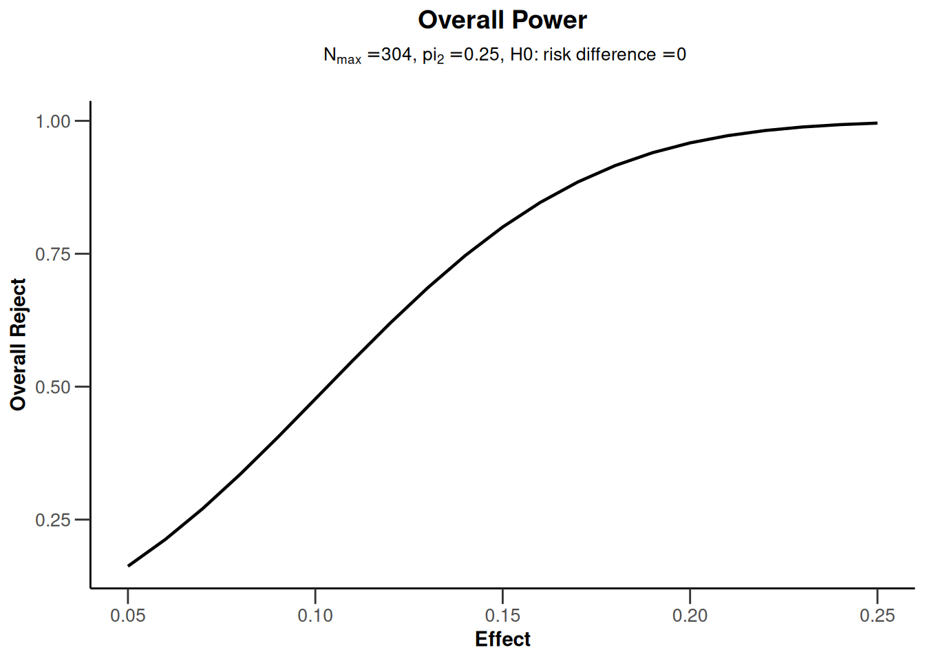
Sample size calculation for a non-inferiority trial with two groups without interim analyses
For non-inferiority trials, sample size calculation proceeds in the same fashion as for superiority trials except that the role of the null and the alternative hypothesis are reversed. I.e., in this case, the non-inferiority margin \(\Delta\) corresponds to the treatment effect under the null hypothesis (thetaH0) which one aims to reject. Testing in non-inferiority trials is always one-sided. In the following example, we set the non-inferiority margin to \(\Delta = 0.1\), meaning that the alternative hypothesis consists of risk differences pi1 - pi2 < 0.1. Note that this means that the event of interest is unfavorable (e.g., a treatment failure), in contrast to the above example.
# Example: Sample size for a non-inferiority trial
# Assume pi(control) = pi(intervention) = 0.2
# Test H0: pi1 - pi2 = 0.1 (risk increase in intervention >= Delta = 0.1)
# vs. H1: pi1 - pi2 < 0.1
getSampleSizeRates(
    pi2 = 0.2,
    pi1 = 0.2,
    thetaH0 = 0.1,
    sided = 1,
    alpha = 0.025,
    beta = 0.2
) |>
    summary()
Sample size calculation for a binary endpoint
Fixed sample analysis, one-sided significance level 2.5%, power 80%. The results were calculated for a two-sample test for rates (normal approximation), H0: pi(1) - pi(2) = 0.1, H1: pi(1) = 0.2, control rate pi(2) = 0.2.
| Stage | Fixed |
|---|---|
| Stage level (one-sided) | 0.0250 |
| Efficacy boundary (z-value scale) | 1.960 |
| Efficacy boundary (t) | 0.028 |
| Number of subjects | 508.4 |
Legend:
- (t): treatment effect scale
Sample size calculation for a single arm trial without interim analyses
The function getSampleSizeRates() allows to set the number of groups (which is 2 by default) to 1 for the design of single-arm trials. The probability under the null hypothesis can be specified with the argument thetaH0and the specific alternative hypothesis which is used for the sample size calculation is provided using the argument pi1. The sample size calculation can be based either on a normal approximation (normalApproximation = TRUE, the default) or on exact binomial probabilities (normalApproximation = FALSE).
# Example: Sample size for a single arm trial which tests
# H0: pi = 0.1 vs. H1: pi = 0.25
# (use conservative exact binomial calculation)
getSampleSizeRates(
    groups = 1,
    thetaH0 = 0.1,
    pi1 = 0.25,
    normalApproximation = FALSE,
    sided = 1,
    alpha = 0.025,
    beta = 0.2
) |>
  summary()
Sample size calculation for a binary endpoint
Fixed sample analysis, one-sided significance level 2.5%, power 80%. The results were calculated for a one-sample test for rates (exact test, conservative solution), H0: pi = 0.1, H1: pi = 0.25.
| Stage | Fixed |
|---|---|
| Stage level (one-sided) | 0.0250 |
| Efficacy boundary (z-value scale) | 1.960 |
| Efficacy boundary (t) | 0.181 |
| Number of subjects | 53.0 |
Legend:
- (t): treatment effect scale
Sample size calculation for group sequential designs
Sample size calculation for a group sequential trial is performed in two steps:
- Define the (abstract) group sequential design using the function
getDesignGroupSequential(). For details regarding this step, see the vignette Defining group sequential boundaries with rpact. - Calculate sample size for the binary endpoint by feeding the abstract design into the function
getSampleSizeRates(). Note that the power \(1 - \beta\) needs to be defined in the design function via the type II errorbeta, and not ingetSampleSizeRates().
In general, rpact supports both one-sided and two-sided group sequential designs. However, if futility boundaries are specified, only one-sided tests are permitted.
R code for a simple example is provided below:
# Example: Group-sequential design with  O'Brien & Fleming type alpha-spending and
# one interim at 60% information
design <- getDesignGroupSequential(
    sided = 1,
    alpha = 0.025,
    beta = 0.2,
    informationRates = c(0.6, 1),
    typeOfDesign = "asOF"
)

# Sample size calculation assuming event probabilities are 25% in control
# (pi2 = 0.25) vs 40% (pi1 = 0.4) in intervention
sampleSizeResultGS <- getSampleSizeRates(
  design,
  pi2 = 0.25,
  pi1 = 0.4)
# Standard rpact output (sample size object only, not design object)
sampleSizeResultGS
Design plan parameters and output for rates
Design parameters
- Information rates: 0.600, 1.000
- Critical values: 2.669, 1.981
- Futility bounds (non-binding): -Inf
- Cumulative alpha spending: 0.003808, 0.025000
- Local one-sided significance levels: 0.003808, 0.023798
- Significance level: 0.0250
- Type II error rate: 0.2000
- Test: one-sided
User defined parameters
- Assumed treatment rate: 0.400
- Assumed control rate: 0.250
Default parameters
- Risk ratio: FALSE
- Theta H0: 0
- Normal approximation: TRUE
- Treatment groups: 2
- Planned allocation ratio: 1
Sample size and output
- Direction upper: TRUE
- Maximum number of subjects: 306.3
- Maximum number of subjects (1): 153.2
- Maximum number of subjects (2): 153.2
- Number of subjects [1]: 183.8
- Number of subjects [2]: 306.3
- Reject per stage [1]: 0.3123
- Reject per stage [2]: 0.4877
- Early stop: 0.3123
- Expected number of subjects under H0: 305.9
- Expected number of subjects under H0/H1: 299.3
- Expected number of subjects under H1: 268.1
- Critical values (treatment effect scale) [1]: 0.187
- Critical values (treatment effect scale) [2]: 0.104
Legend
- (i): values of treatment arm i
- [k]: values at stage k
We see from the output that the maximum number of subjects for the trial per treatment group is 153.2 patients. Rounding up, this yields 154 patients per treatment group and a total maximum sample size of 308 patients. The maximum sample size of the two-stage design is thus only marginally larger than the maximum sample size of the fixed design with the same parameters (which was 304 patients).
The summary() command produces the output
sampleSizeResultGS |> summary()Sample size calculation for a binary endpoint
Sequential analysis with a maximum of 2 looks (group sequential design), one-sided overall significance level 2.5%, power 80%. The results were calculated for a two-sample test for rates (normal approximation), H0: pi(1) - pi(2) = 0, H1: pi(1) = 0.4, control rate pi(2) = 0.25.
| Stage | 1 | 2 |
|---|---|---|
| Planned information rate | 60% | 100% |
| Cumulative alpha spent | 0.0038 | 0.0250 |
| Stage levels (one-sided) | 0.0038 | 0.0238 |
| Efficacy boundary (z-value scale) | 2.669 | 1.981 |
| Efficacy boundary (t) | 0.187 | 0.104 |
| Cumulative power | 0.3123 | 0.8000 |
| Number of subjects | 183.8 | 306.3 |
| Expected number of subjects under H1 | 268.1 | |
| Exit probability for efficacy (under H0) | 0.0038 | |
| Exit probability for efficacy (under H1) | 0.3123 |
Legend:
- (t): treatment effect scale
System: rpact 4.2.0, R version 4.4.3 (2025-02-28), platform: x86_64-pc-linux-gnu
To cite R in publications use:
R Core Team (2025). R: A Language and Environment for Statistical Computing. R Foundation for Statistical Computing, Vienna, Austria. https://www.R-project.org/.
To cite package ‘rpact’ in publications use:
Wassmer G, Pahlke F (2025). rpact: Confirmatory Adaptive Clinical Trial Design and Analysis. doi:10.32614/CRAN.package.rpact https://doi.org/10.32614/CRAN.package.rpact, R package version 4.2.0, https://cran.r-project.org/package=rpact.