library(rpact)
packageVersion("rpact") # version should be version 3.0 or laterAnalysis of a Multi-Arm Design with a Binary Endpoint using rpact
Analysis
Rates
Multi-arm
This document shows how to analyse and interpret multi-arm designs for testing proportions with rpact.
Introduction
This vignette provides examples of how to analyse a trial with multiple arms and a binary endpoint. It shows how to calculate the conditional power at a given stage and how to select/deselect treatment arms. For designs with multiple arms, rpact enables the analysis using the closed combination testing principle. For a description of the methodology please refer to Part III of the book “Group Sequential and Confirmatory Adaptive Designs in Clinical Trials” (Wassmer and Brannath, 2016).
Suppose the trial was conducted as a multi-arm multi-stage trial with three active treatments arms and a control arm when the trial started. In the interim stages, it should be possible to de-select treatment arms if their treatment effect is likely too small to show significance - assuming reasonable sample size - at the end of the trial. This should hold true even if a certain sample size increase was taken into account. For this vignette, the considered endpoint is a failure (i.e., binary) and it is intended to test each active arm against a common control. This is to test the hypotheses \[ H_{0i}:\pi_{\text{arm}i} = \pi_\text{control} \qquad\text{against} \qquad H_{1i}:\pi_{\text{arm}i} < \pi_\text{control}\;, \;i = 1,2,3\,,\] in the many-to-one comparisons setting. That is, it is intended to show that the failure rate is smaller in active arms as compared to control and so the power is directed towards negative values of \(\pi_{\text{arm}i} - \pi_\text{control}\).
Create the design
First, load the rpact package
[1] '4.2.0'In rpact, we first have to select the combination test with the corresponding stopping boundaries to be used in the closed testing procedure. We choose a design with critical values within the Wang & Tsiatis \(\Delta\)-class of boundaries with \(\Delta = 0.25\). Planning two interim stages and a final stage, assuming equally sized stages, the design is defined through
designIN <- getDesignInverseNormal(
    kMax = 3,
    alpha = 0.025,
    typeOfDesign = "WT",
    deltaWT = 0.25
)
designIN |> summary()
Sequential analysis with a maximum of 3 looks (inverse normal combination test design)
Wang & Tsiatis Delta class design (deltaWT = 0.25), one-sided overall significance level 2.5%, power 80%, undefined endpoint, inflation factor 1.0544, ASN H1 0.8202, ASN H01 0.9966, ASN H0 1.0489.
| Stage | 1 | 2 | 3 |
|---|---|---|---|
| Fixed weight | 0.577 | 0.577 | 0.577 |
| Cumulative alpha spent | 0.0031 | 0.0124 | 0.0250 |
| Stage levels (one-sided) | 0.0031 | 0.0106 | 0.0186 |
| Efficacy boundary (z-value scale) | 2.741 | 2.305 | 2.083 |
| Cumulative power | 0.1400 | 0.5262 | 0.8000 |
This definition fixes the weights in the combination test which are the same over the three stages. This is a reasonable choice although the amount of information seems to be not the same over the stages (see Wassmer, 2010).
Analysis
First stage
In each of the four arms (three treatment arms and one control arm), subjects were randomized such that around 40 subjects per arm will be observed. Assume that the following actual sample sizes and failures in the control and the three experimental treatment arms were obtained for the first stage of the trial:
| Arm | n | Failures |
|---|---|---|
| Active 1 | 42 | 7 |
| Active 2 | 39 | 8 |
| Active 3 | 38 | 14 |
| Control | 41 | 18 |
These data are defined as an rpact dataset with the function getDataset() for the later use in getAnalysisResults() through
dataRates <- getDataset(
    events1      =  7,
    events2      =  8,
    events3      = 14,
    events4      = 18,
    sampleSizes1 = 42,
    sampleSizes2 = 39,
    sampleSizes3 = 38,
    sampleSizes4 = 41
)
That is, you can use the getDataset() function in the usual way and simply extend it to the multiple treatment arms situation. Note that the arm with the highest index always refers to the control group. For the control group, specifically, it is mandatory to enter values over all stages. As we will see below, it is possible to omit information of de-selected active arms.
Using
getAnalysisResults(
    design = designIN,
    dataInput = dataRates,
    directionUpper = FALSE
) |>
    summary()
one obtains the test results for the first stage of this trial (note the directionUpper = FALSE specification that yields small \(p\)-values for negative test statistics):
Multi-arm analysis results for a binary endpoint (3 active arms vs. control)
Sequential analysis with 3 looks (inverse normal combination test design), one-sided overall significance level 2.5%. The results were calculated using a multi-arm test for rates, Dunnett intersection test, normal approximation test. H0: pi(i) - pi(control) = 0 against H1: pi(i) - pi(control) < 0.
| Stage | 1 | 2 | 3 |
|---|---|---|---|
| Fixed weight | 0.577 | 0.577 | 0.577 |
| Cumulative alpha spent | 0.0031 | 0.0124 | 0.0250 |
| Stage levels (one-sided) | 0.0031 | 0.0106 | 0.0186 |
| Efficacy boundary (z-value scale) | 2.741 | 2.305 | 2.083 |
| Cumulative effect size (1) | -0.272 | ||
| Cumulative effect size (2) | -0.234 | ||
| Cumulative effect size (3) | -0.071 | ||
| Cumulative treatment rate (1) | 0.167 | ||
| Cumulative treatment rate (2) | 0.205 | ||
| Cumulative treatment rate (3) | 0.368 | ||
| Cumulative control rate | 0.439 | ||
| Stage-wise test statistic (1) | -2.704 | ||
| Stage-wise test statistic (2) | -2.233 | ||
| Stage-wise test statistic (3) | -0.639 | ||
| Stage-wise p-value (1) | 0.0034 | ||
| Stage-wise p-value (2) | 0.0128 | ||
| Stage-wise p-value (3) | 0.2615 | ||
| Adjusted stage-wise p-value (1, 2, 3) | 0.0095 | ||
| Adjusted stage-wise p-value (1, 2) | 0.0066 | ||
| Adjusted stage-wise p-value (1, 3) | 0.0066 | ||
| Adjusted stage-wise p-value (2, 3) | 0.0239 | ||
| Adjusted stage-wise p-value (1) | 0.0034 | ||
| Adjusted stage-wise p-value (2) | 0.0128 | ||
| Adjusted stage-wise p-value (3) | 0.2615 | ||
| Overall adjusted test statistic (1, 2, 3) | 2.346 | ||
| Overall adjusted test statistic (1, 2) | 2.480 | ||
| Overall adjusted test statistic (1, 3) | 2.480 | ||
| Overall adjusted test statistic (2, 3) | 1.980 | ||
| Overall adjusted test statistic (1) | 2.704 | ||
| Overall adjusted test statistic (2) | 2.233 | ||
| Overall adjusted test statistic (3) | 0.639 | ||
| Test action: reject (1) | FALSE | ||
| Test action: reject (2) | FALSE | ||
| Test action: reject (3) | FALSE | ||
| Conditional rejection probability (1) | 0.2647 | ||
| Conditional rejection probability (2) | 0.1708 | ||
| Conditional rejection probability (3) | 0.0202 | ||
| 95% repeated confidence interval (1) | [-0.541; 0.038] | ||
| 95% repeated confidence interval (2) | [-0.514; 0.089] | ||
| 95% repeated confidence interval (3) | [-0.384; 0.259] | ||
| Repeated p-value (1) | 0.0519 | ||
| Repeated p-value (2) | 0.0948 | ||
| Repeated p-value (3) | 0.4568 |
Legend:
- (i): results of treatment arm i vs. control arm
- (i, j, …): comparison of treatment arms ‘i, j, …’ vs. control arm
First of all, at the first interim no hypothesis can be rejected with the closed combination test. This is seen from the Test action: reject (i) variable. It is remarkable, however, that the \(p\)-value for the comparison of treatment arm 1 against control (p = 0.0034) is quite small and even the \(p\)-value for the global intersection is (p(1, 2, 3) = 0.0095) is not too far from showing significance. It is important to know that, by default, the Dunnett many-to-one comparison test for binary data is used as the test for the intersection hypotheses, and the approximate pairwise score test (which is the signed square root of the \(\chi^2\) test) is used for the calculation of the separate \(p\)-values. Note that in this presentation, the intersection test for the whole closed system of hypotheses is provided such that the closed test can completely be reproduced.
The repeated \(p\)-values (0.0519, 0.0948, and 0.4568, respectively) precisely correspond with the test decision meaning that a repeated \(p\)-value is smaller or equal to the overall significance level (0.025) if and only if the corresponding hypothesis can be rejected at the considered stage. This direct correspondence is not generally true for the repeated confidence intervals (i.e., they can contain the value zero although the null hypothesis can be rejected), but it is true for the situation at hand. The repeated confidence intervals can be displayed with the plot(type = 2) command by
results |> plot(type = 2)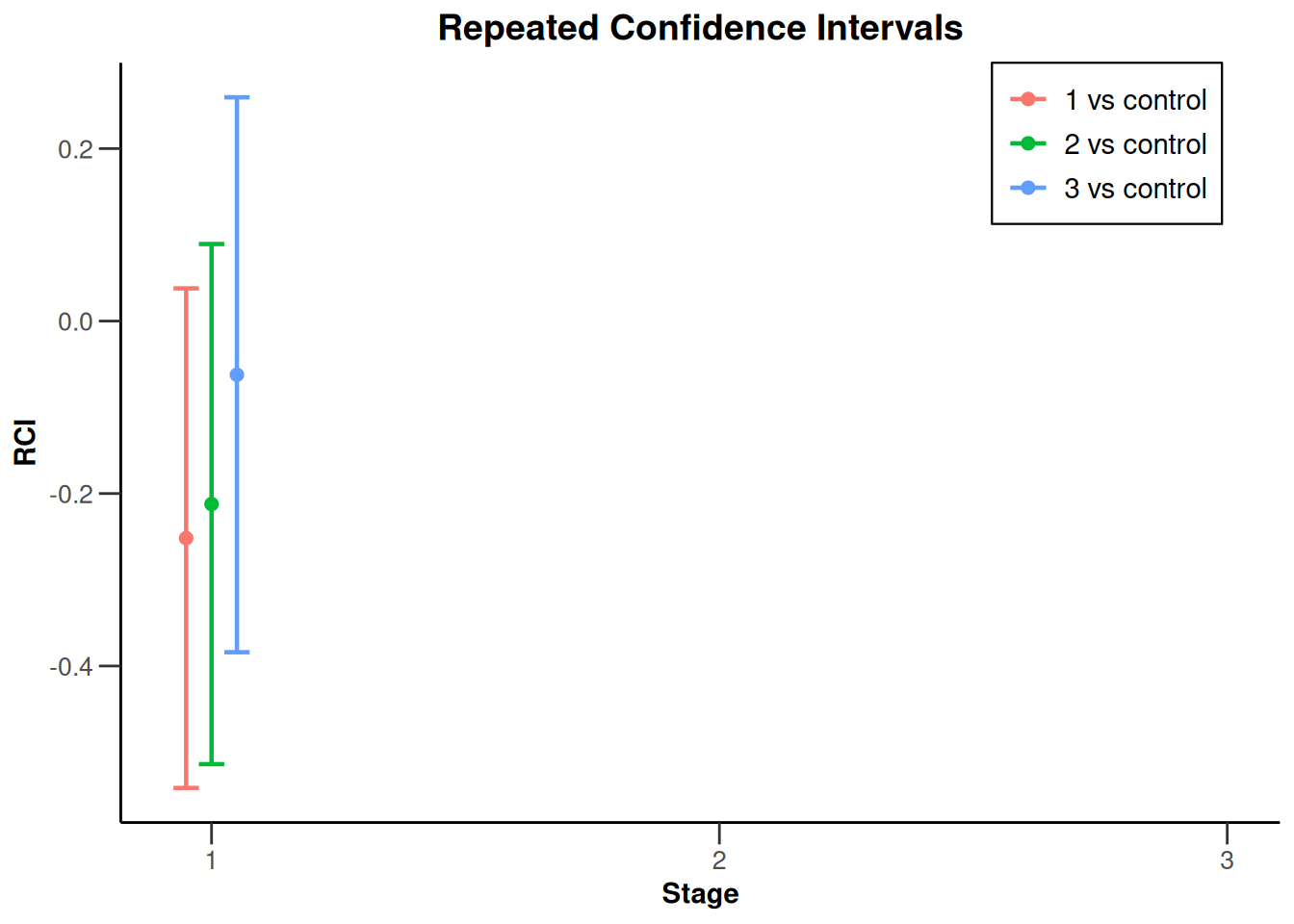
For assessing the conditional power, a sample size specification for the remaining stages needs to be done. We assume that around 80 subjects will be obtained per considered comparison and per stage (i.e., 40 subjects per stage for each considered treatment group and 40 subjects per stage for the control arm). Use ?getAnalysisResults() for further information about how to specify the parameter nPlanned. Assuming 80 subjects you have to re-run (options("rpact.summary.output.size" = "small") reduces the output of the summary)
options("rpact.summary.output.size" = "small")
getAnalysisResults(
    design = designIN,
    dataInput = dataRates,
    directionUpper = FALSE,
    nPlanned = c(80, 80)
) |>
    summary()
to obtain
Multi-arm analysis results for a binary endpoint (3 active arms vs. control)
Sequential analysis with 3 looks (inverse normal combination test design), one-sided overall significance level 2.5%. The results were calculated using a multi-arm test for rates, Dunnett intersection test, normal approximation test. H0: pi(i) - pi(control) = 0 against H1: pi(i) - pi(control) < 0. The conditional power calculation with planned sample size is based on overall treatment rate: pi(1) = 0.17, pi(2) = 0.21, pi(3) = 0.37 and overall control rate = 0.439.
| Stage | 1 | 2 | 3 |
|---|---|---|---|
| Fixed weight | 0.577 | 0.577 | 0.577 |
| Cumulative alpha spent | 0.0031 | 0.0124 | 0.0250 |
| Stage levels (one-sided) | 0.0031 | 0.0106 | 0.0186 |
| Efficacy boundary (z-value scale) | 2.741 | 2.305 | 2.083 |
| Cumulative effect size (1) | -0.272 | ||
| Cumulative effect size (2) | -0.234 | ||
| Cumulative effect size (3) | -0.071 | ||
| Stage-wise test statistic (1) | -2.704 | ||
| Stage-wise test statistic (2) | -2.233 | ||
| Stage-wise test statistic (3) | -0.639 | ||
| Stage-wise p-value (1) | 0.0034 | ||
| Stage-wise p-value (2) | 0.0128 | ||
| Stage-wise p-value (3) | 0.2615 | ||
| Test action: reject (1) | FALSE | ||
| Test action: reject (2) | FALSE | ||
| Test action: reject (3) | FALSE | ||
| Conditional rejection probability (1) | 0.2647 | ||
| Conditional rejection probability (2) | 0.1708 | ||
| Conditional rejection probability (3) | 0.0202 | ||
| Planned sample size | 80 | 80 | |
| Conditional power (1) | 0.9672 | 0.9990 | |
| Conditional power (2) | 0.8438 | 0.9846 | |
| Conditional power (3) | 0.0239 | 0.1229 | |
| 95% repeated confidence interval (1) | [-0.541; 0.038] | ||
| 95% repeated confidence interval (2) | [-0.514; 0.089] | ||
| 95% repeated confidence interval (3) | [-0.384; 0.259] | ||
| Repeated p-value (1) | 0.0519 | ||
| Repeated p-value (2) | 0.0948 | ||
| Repeated p-value (3) | 0.4568 |
Legend:
- (i): results of treatment arm i vs. control arm
The Conditional power (i) variable shows very high power (esp. for the final stage) for treatment arms 1 and 2, but not for arm 3. Note that the conditional power is calculated under the assumption that the observed rates are the true rates. This can be changed, however, by setting piControl and/or piTreatments equal to the desired values (piTreatments can even be a vector specifying one rate per active treatment arm), e.g.,
results <- getAnalysisResults(
    design = designIN,
    dataInput = dataRates,
    directionUpper = FALSE,
    nPlanned = c(80, 80),
    piTreatments = c(0.17, 0.2, 0.37),
    piControl = 0.44
)
results |> summary()
Multi-arm analysis results for a binary endpoint (3 active arms vs. control)
Sequential analysis with 3 looks (inverse normal combination test design), one-sided overall significance level 2.5%. The results were calculated using a multi-arm test for rates, Dunnett intersection test, normal approximation test. H0: pi(i) - pi(control) = 0 against H1: pi(i) - pi(control) < 0. The conditional power calculation with planned sample size is based on assumed treatment rate: pi(1) = 0.17, pi(2) = 0.2, pi(3) = 0.37 and assumed control rate = 0.44.
| Stage | 1 | 2 | 3 |
|---|---|---|---|
| Fixed weight | 0.577 | 0.577 | 0.577 |
| Cumulative alpha spent | 0.0031 | 0.0124 | 0.0250 |
| Stage levels (one-sided) | 0.0031 | 0.0106 | 0.0186 |
| Efficacy boundary (z-value scale) | 2.741 | 2.305 | 2.083 |
| Cumulative effect size (1) | -0.272 | ||
| Cumulative effect size (2) | -0.234 | ||
| Cumulative effect size (3) | -0.071 | ||
| Stage-wise test statistic (1) | -2.704 | ||
| Stage-wise test statistic (2) | -2.233 | ||
| Stage-wise test statistic (3) | -0.639 | ||
| Stage-wise p-value (1) | 0.0034 | ||
| Stage-wise p-value (2) | 0.0128 | ||
| Stage-wise p-value (3) | 0.2615 | ||
| Test action: reject (1) | FALSE | ||
| Test action: reject (2) | FALSE | ||
| Test action: reject (3) | FALSE | ||
| Conditional rejection probability (1) | 0.2647 | ||
| Conditional rejection probability (2) | 0.1708 | ||
| Conditional rejection probability (3) | 0.0202 | ||
| Planned sample size | 80 | 80 | |
| Conditional power (1) | 0.9648 | 0.9988 | |
| Conditional power (2) | 0.8594 | 0.9879 | |
| Conditional power (3) | 0.0235 | 0.1213 | |
| 95% repeated confidence interval (1) | [-0.541; 0.038] | ||
| 95% repeated confidence interval (2) | [-0.514; 0.089] | ||
| 95% repeated confidence interval (3) | [-0.384; 0.259] | ||
| Repeated p-value (1) | 0.0519 | ||
| Repeated p-value (2) | 0.0948 | ||
| Repeated p-value (3) | 0.4568 |
Legend:
- (i): results of treatment arm i vs. control arm
Note that the title of the summary describes the situation under which the conditional power calculation is performed.
results |> plot(
    type = 1,
    piTreatmentRange = c(0, 0.5),
    legendPosition = 3)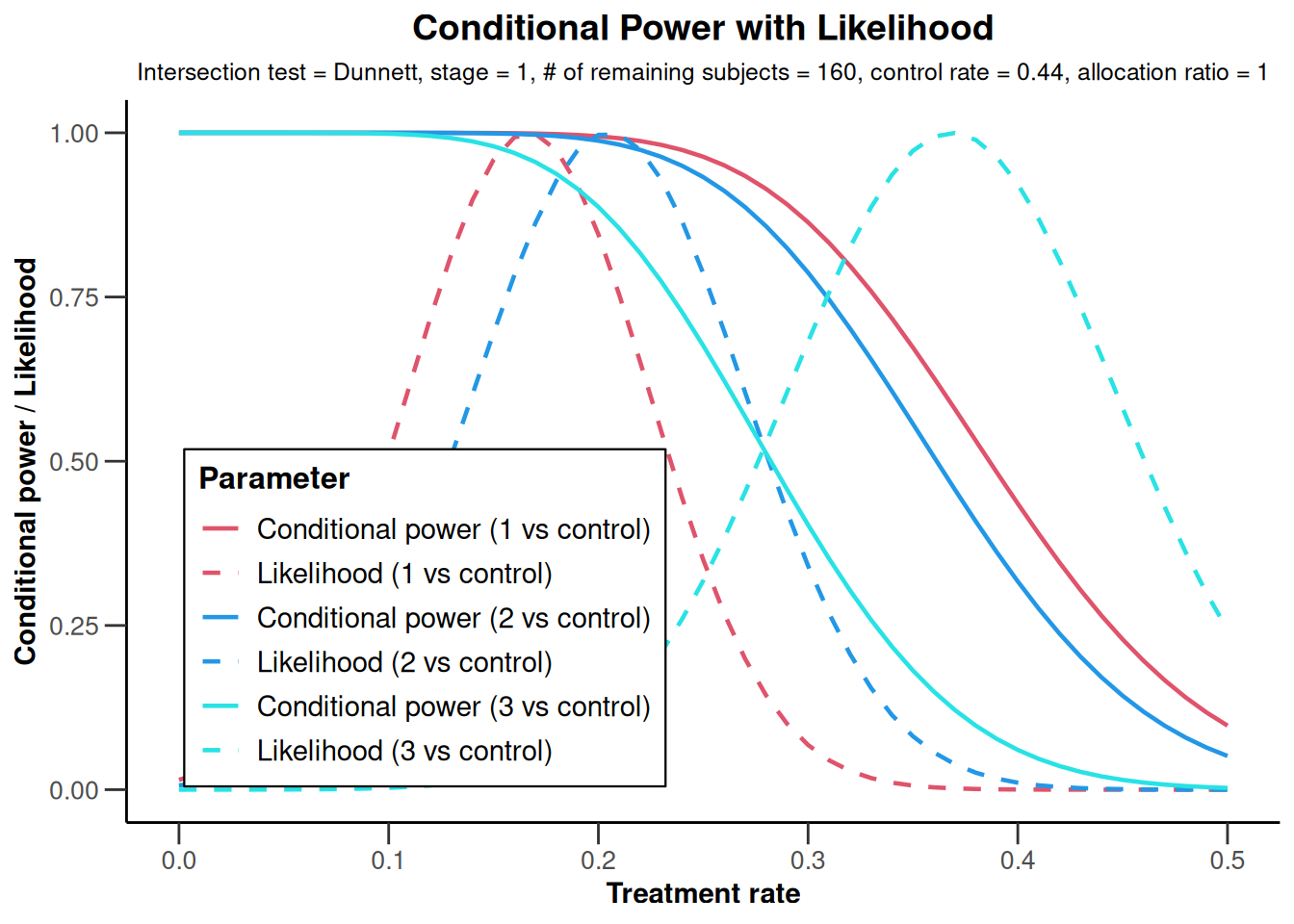
NULLAltogether, based on the results of the first interim the decision to drop treatment arm 3 and to recruit further 40 patients to each treatment arms 1 and 2 (and to the control group) was taken.
Second stage
Also for the second stage, in each of the remaining treatment arms and the control arm, subjects were randomized such that around 40 subjects per arm will be observed. Assume the following failures and actual sample sizes in the control and the two remaining arms:
| Arm | n | Failures |
|---|---|---|
| Active 1 | 37 | 9 |
| Active 2 | 41 | 13 |
| Active 3 | ||
| Control | 42 | 19 |
With getDataset(), these data for the second stage are appended to the first stage data as follows:
dataRates <- getDataset(
    events1 = c(7, 9),
    events2 = c(8, 13),
    events3 = c(14, NA),
    events4 = c(18, 19),
    sampleSizes1 = c(42, 37),
    sampleSizes2 = c(39, 41),
    sampleSizes3 = c(38, NA),
    sampleSizes4 = c(41, 42)
)
and the stage 2 results are obtained with getAnalysisResults() as above. Printing a summary of the analysis results yields:
Multi-arm analysis results for a binary endpoint (3 active arms vs. control)
Sequential analysis with 3 looks (inverse normal combination test design), one-sided overall significance level 2.5%. The results were calculated using a multi-arm test for rates, Dunnett intersection test, normal approximation test. H0: pi(i) - pi(control) = 0 against H1: pi(i) - pi(control) < 0.
| Stage | 1 | 2 | 3 |
|---|---|---|---|
| Fixed weight | 0.577 | 0.577 | 0.577 |
| Cumulative alpha spent | 0.0031 | 0.0124 | 0.0250 |
| Stage levels (one-sided) | 0.0031 | 0.0106 | 0.0186 |
| Efficacy boundary (z-value scale) | 2.741 | 2.305 | 2.083 |
| Cumulative effect size (1) | -0.272 | -0.243 | |
| Cumulative effect size (2) | -0.234 | -0.183 | |
| Cumulative effect size (3) | -0.071 | ||
| Cumulative treatment rate (1) | 0.167 | 0.203 | |
| Cumulative treatment rate (2) | 0.205 | 0.262 | |
| Cumulative treatment rate (3) | 0.368 | ||
| Cumulative control rate | 0.439 | 0.446 | |
| Stage-wise test statistic (1) | -2.704 | -1.939 | |
| Stage-wise test statistic (2) | -2.233 | -1.266 | |
| Stage-wise test statistic (3) | -0.639 | ||
| Stage-wise p-value (1) | 0.0034 | 0.0262 | |
| Stage-wise p-value (2) | 0.0128 | 0.1027 | |
| Stage-wise p-value (3) | 0.2615 | ||
| Adjusted stage-wise p-value (1, 2, 3) | 0.0095 | 0.0478 | |
| Adjusted stage-wise p-value (1, 2) | 0.0066 | 0.0478 | |
| Adjusted stage-wise p-value (1, 3) | 0.0066 | 0.0262 | |
| Adjusted stage-wise p-value (2, 3) | 0.0239 | 0.1027 | |
| Adjusted stage-wise p-value (1) | 0.0034 | 0.0262 | |
| Adjusted stage-wise p-value (2) | 0.0128 | 0.1027 | |
| Adjusted stage-wise p-value (3) | 0.2615 | ||
| Overall adjusted test statistic (1, 2, 3) | 2.346 | 2.837 | |
| Overall adjusted test statistic (1, 2) | 2.480 | 2.932 | |
| Overall adjusted test statistic (1, 3) | 2.480 | 3.125 | |
| Overall adjusted test statistic (2, 3) | 1.980 | 2.295 | |
| Overall adjusted test statistic (1) | 2.704 | 3.283 | |
| Overall adjusted test statistic (2) | 2.233 | 2.474 | |
| Overall adjusted test statistic (3) | 0.639 | ||
| Test action: reject (1) | FALSE | TRUE | |
| Test action: reject (2) | FALSE | FALSE | |
| Test action: reject (3) | FALSE | FALSE | |
| Conditional rejection probability (1) | 0.2647 | 0.6572 | |
| Conditional rejection probability (2) | 0.1708 | 0.3589 | |
| Conditional rejection probability (3) | 0.0202 | ||
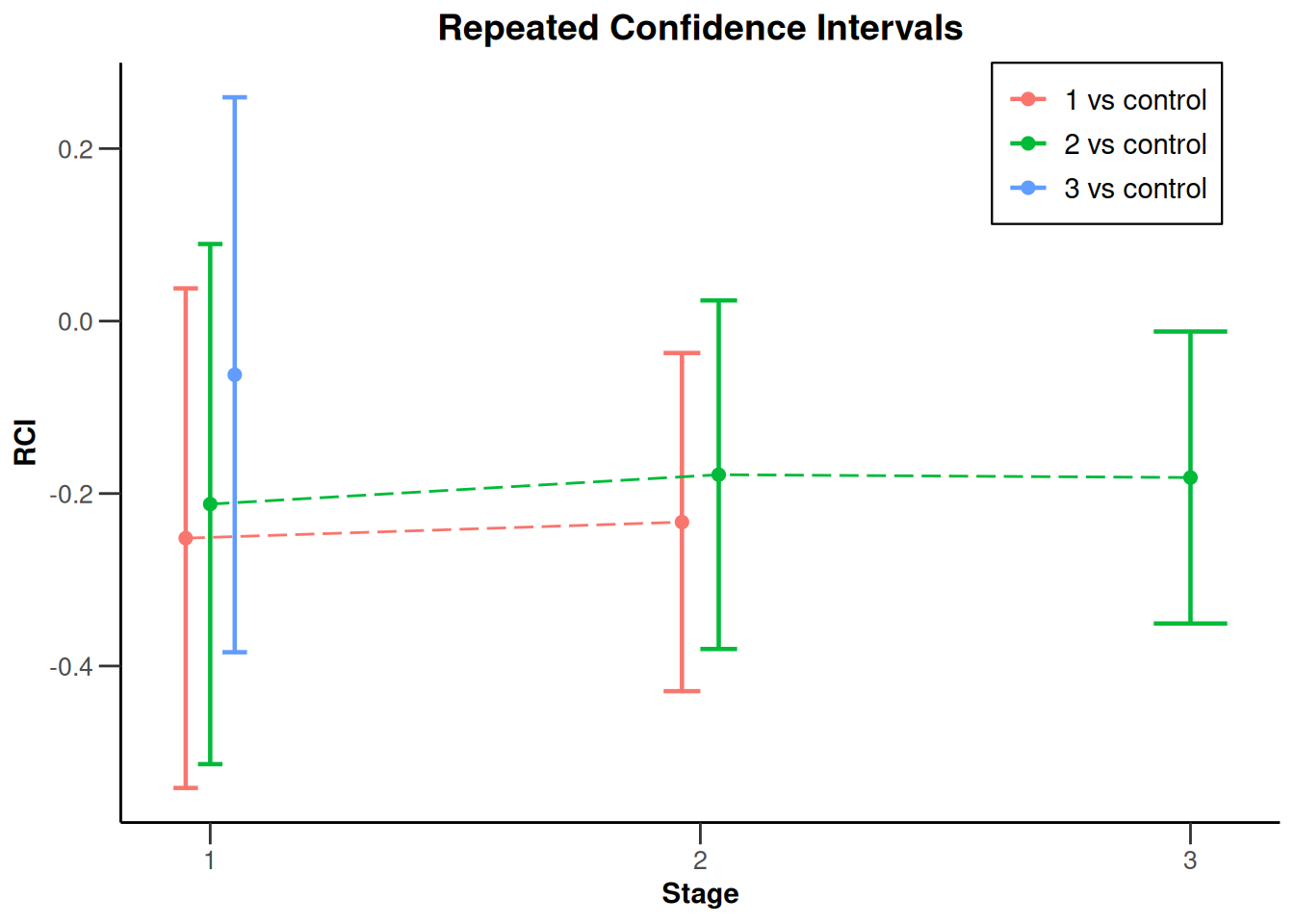
| 95% repeated confidence interval (1) | [-0.541; 0.038] | [-0.429; -0.037] | |
| 95% repeated confidence interval (2) | [-0.514; 0.089] | [-0.380; 0.024] | |
| 95% repeated confidence interval (3) | [-0.384; 0.259] | ||
| Repeated p-value (1) | 0.0519 | 0.0065 | |
| Repeated p-value (2) | 0.0948 | 0.0256 | |
| Repeated p-value (3) | 0.4568 |
Legend:
- (i): results of treatment arm i vs. control arm
- (i, j, …): comparison of treatment arms ‘i, j, …’ vs. control arm
Treatment arm 1 is significantly better than control, stated by Test action: reject (1), and reflected in both Repeated $p$-value (1) falling below 0.025 and the Repeated confidence interval (1) excluding 0. For treatment arm 2, however, significance could not be shown, although both, the global intersection hypothesis and the single hypothesis referring to treatment arm 2, can be rejected with the corresponding combination test. The reason for non-significance is the overall adjusted test statistic for testing \(H_{02}\cap H_{03}\) which is 2.295 < 2.305.
In order to show significance also for treatment arm 2, one might calculate the power if the sample size of the final stage was reduced to 20 subjects per considered arm (treatment arm 2 and control). This is achieved through
options("rpact.summary.output.size" = "small") # small, medium, large
results <- getAnalysisResults(
    design = designIN,
    dataInput = dataRates,
    directionUpper = FALSE,
    nPlanned = 40
)
results |> summary()
Multi-arm analysis results for a binary endpoint (3 active arms vs. control)
Sequential analysis with 3 looks (inverse normal combination test design), one-sided overall significance level 2.5%. The results were calculated using a multi-arm test for rates, Dunnett intersection test, normal approximation test. H0: pi(i) - pi(control) = 0 against H1: pi(i) - pi(control) < 0. The conditional power calculation with planned sample size is based on overall treatment rate: pi(1) = 0.2, pi(2) = 0.26, pi(3) = NA and overall control rate = 0.446.
| Stage | 1 | 2 | 3 |
|---|---|---|---|
| Fixed weight | 0.577 | 0.577 | 0.577 |
| Cumulative alpha spent | 0.0031 | 0.0124 | 0.0250 |
| Stage levels (one-sided) | 0.0031 | 0.0106 | 0.0186 |
| Efficacy boundary (z-value scale) | 2.741 | 2.305 | 2.083 |
| Cumulative effect size (1) | -0.272 | -0.243 | |
| Cumulative effect size (2) | -0.234 | -0.183 | |
| Cumulative effect size (3) | -0.071 | ||
| Stage-wise test statistic (1) | -2.704 | -1.939 | |
| Stage-wise test statistic (2) | -2.233 | -1.266 | |
| Stage-wise test statistic (3) | -0.639 | ||
| Stage-wise p-value (1) | 0.0034 | 0.0262 | |
| Stage-wise p-value (2) | 0.0128 | 0.1027 | |
| Stage-wise p-value (3) | 0.2615 | ||
| Test action: reject (1) | FALSE | TRUE | |
| Test action: reject (2) | FALSE | FALSE | |
| Test action: reject (3) | FALSE | FALSE | |
| Conditional rejection probability (1) | 0.2647 | 0.6572 | |
| Conditional rejection probability (2) | 0.1708 | 0.3589 | |
| Conditional rejection probability (3) | 0.0202 | ||
| Planned sample size | 40 | ||
| Conditional power (1) | 0.9830 | ||
| Conditional power (2) | 0.8069 | ||
| Conditional power (3) | |||
| 95% repeated confidence interval (1) | [-0.541; 0.038] | [-0.429; -0.037] | |
| 95% repeated confidence interval (2) | [-0.514; 0.089] | [-0.380; 0.024] | |
| 95% repeated confidence interval (3) | [-0.384; 0.259] | ||
| Repeated p-value (1) | 0.0519 | 0.0065 | |
| Repeated p-value (2) | 0.0948 | 0.0256 | |
| Repeated p-value (3) | 0.4568 |
Legend:
- (i): results of treatment arm i vs. control arm
showing that conditional power might be reduced to around 80% if the sample size was decreased. However, as showing in this graph
NULLthis is predominantly due to the relatively large observed overall failure rate in stage 2. Assuming a failure rate of (say) 20% yields conditional power of 91.1% which is obtained from
results <- getAnalysisResults(
    design = designIN,
    dataInput = dataRates,
    directionUpper = FALSE,
    nPlanned = 40,
    piTreatments = 0.2
)
round(100 * results$conditionalPower[2, 3], 1)
Therefore, it might be reasonable to drop treatment arm 1 (for which significance was already shown) and compare treatment arm 2 only against control in the final stage.
Final stage
Assume the following sample sizes and failures for the final stage where only (additional) active arm 2 and control data were obtained.
| Arm | n | Failures |
|---|---|---|
| Active 1 | ||
| Active 2 | 18 | 7 |
| Active 3 | ||
| Control | 19 | 11 |
These data for the final stage are entered as follows:
dataRates <- getDataset(
    events1 = c(7, 9, NA),
    events2 = c(8, 13, 7),
    events3 = c(14, NA, NA),
    events4 = c(18, 19, 11),
    sampleSizes1 = c(42, 37, NA),
    sampleSizes2 = c(39, 41, 18),
    sampleSizes3 = c(38, NA, NA),
    sampleSizes4 = c(41, 42, 19)
)
and
results <- getAnalysisResults(
    design = designIN,
    dataInput = dataRates,
    directionUpper = FALSE
)
results |> summary()
provides the results (significance for treatment arm 2 could additionally be shown):
Multi-arm analysis results for a binary endpoint (3 active arms vs. control)
Sequential analysis with 3 looks (inverse normal combination test design), one-sided overall significance level 2.5%. The results were calculated using a multi-arm test for rates, Dunnett intersection test, normal approximation test. H0: pi(i) - pi(control) = 0 against H1: pi(i) - pi(control) < 0.
| Stage | 1 | 2 | 3 |
|---|---|---|---|
| Fixed weight | 0.577 | 0.577 | 0.577 |
| Cumulative alpha spent | 0.0031 | 0.0124 | 0.0250 |
| Stage levels (one-sided) | 0.0031 | 0.0106 | 0.0186 |
| Efficacy boundary (z-value scale) | 2.741 | 2.305 | 2.083 |
| Cumulative effect size (1) | -0.272 | -0.243 | |
| Cumulative effect size (2) | -0.234 | -0.183 | -0.185 |
| Cumulative effect size (3) | -0.071 | ||
| Stage-wise test statistic (1) | -2.704 | -1.939 | |
| Stage-wise test statistic (2) | -2.233 | -1.266 | -1.156 |
| Stage-wise test statistic (3) | -0.639 | ||
| Stage-wise p-value (1) | 0.0034 | 0.0262 | |
| Stage-wise p-value (2) | 0.0128 | 0.1027 | 0.1238 |
| Stage-wise p-value (3) | 0.2615 | ||
| Test action: reject (1) | FALSE | TRUE | TRUE |
| Test action: reject (2) | FALSE | FALSE | TRUE |
| Test action: reject (3) | FALSE | FALSE | FALSE |
| Conditional rejection probability (1) | 0.2647 | 0.6572 | |
| Conditional rejection probability (2) | 0.1708 | 0.3589 | |
| Conditional rejection probability (3) | 0.0202 | ||
| 95% repeated confidence interval (1) | [-0.541; 0.038] | [-0.429; -0.037] | |
| 95% repeated confidence interval (2) | [-0.514; 0.089] | [-0.380; 0.024] | [-0.351; -0.012] |
| 95% repeated confidence interval (3) | [-0.384; 0.259] | ||
| Repeated p-value (1) | 0.0519 | 0.0065 | |
| Repeated p-value (2) | 0.0948 | 0.0256 | 0.0070 |
| Repeated p-value (3) | 0.4568 |
Legend:
- (i): results of treatment arm i vs. control arm
Summarizing the results, plot(results, type = 2, legendPosition = 4) produces a plot of the sequence of repeated confidence intervals over the stages:
Closing remarks
This example describes a range of design modifications, namely selecting treatments arms and performing sample size recalculation for both stages. It is important to recognize that neither the type of adaptation nor the adaptation rule was pre-specified. Despite this, the closed combination test provides control of the experimentwise error rate in the strong sense. To utilize the whole repertoire of possible adaptations, one might also use the conditional rejection probability (i) values in order to completely redefine the design, which includes, for example, to change the number of remaining stages, to change the type of intersection test, or even to add a treatment arm.
Note that in multi-arm designs no final analysis \(p\)-values, confidence intervals, and median unbiased treatment effect estimates are calculated. This is in contrast to the single hypothesis adaptive designs where, using the stage-wise ordering of the sample space, at the final stage such calculations were done with rpact (for example, see the vignette Analysis of a group sequential trial with a survival endpoint).
System: rpact 4.2.0, R version 4.4.3 (2025-02-28), platform: x86_64-pc-linux-gnu
To cite R in publications use:
R Core Team (2025). R: A Language and Environment for Statistical Computing. R Foundation for Statistical Computing, Vienna, Austria. https://www.R-project.org/.
To cite package ‘rpact’ in publications use:
Wassmer G, Pahlke F (2025). rpact: Confirmatory Adaptive Clinical Trial Design and Analysis. doi:10.32614/CRAN.package.rpact https://doi.org/10.32614/CRAN.package.rpact, R package version 4.2.0, https://cran.r-project.org/package=rpact.