library(rpact)
packageVersion("rpact") Using the Inverse Normal Combination Test for Analyzing a Trial with Continuous Endpoint and Potential Sample Size Re-Assessment with rpact
Analysis
Means
This document provides an example for analysing trials with a continuous endpoint and sample size reassessment using rpact.
Define the type of design to be used for the analysis
First, load the rpact package
[1] '4.4.0.9305'In this vignette, we want to illustrate a design where at interim stages we are able to perform data-driven sample size adaptations. For this purpose, we use the inverse normal combination test for combining the \(p\)-values from the stages of the trial. This type of design ensures that the Type I error rate is controlled.
We want to use a three stage design with O`Brien and Fleming boundaries and additionally want to consider futility bounds -0.5 and 0.5 for the test statistics at the first and the second stage, respectively. Accordingly,
# Example of an inverse normal combination test:
designIN <- getDesignInverseNormal(
  futilityBounds = c(-0.5, 0.5)
  )
defines the design to be used for this purpose. By default, this is a design with three stages, equally spaced information rates and one-sided \(\alpha = 0.025\). The critical values can be displayed on the \(z\)-value or the \(p\)-value scale:
designIN |> plot(type = 1)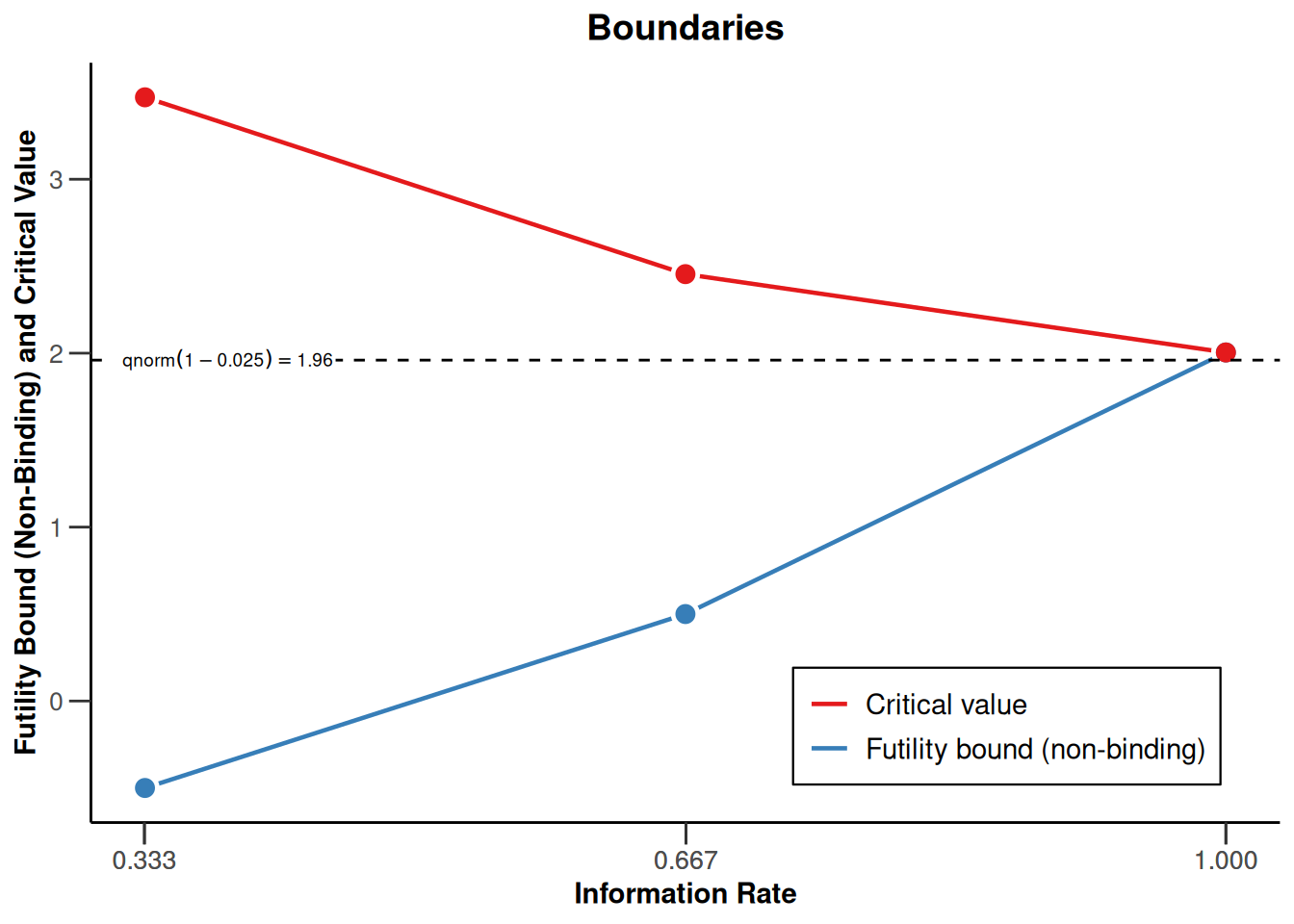
designIN |> plot(type = 3)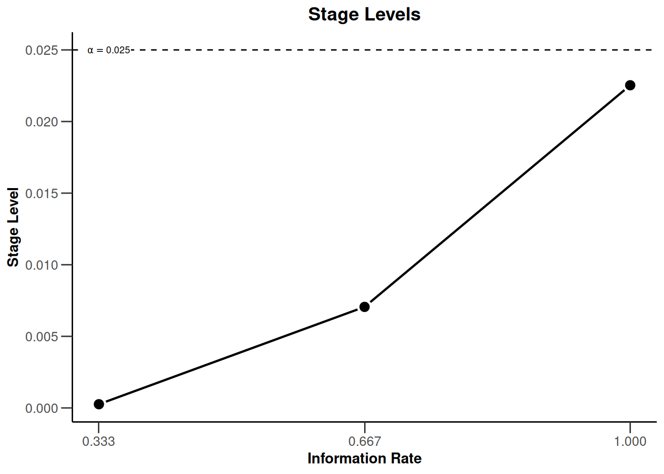
Note that we are using non-binding futility bounds that do not affect the boundaries for the rejection of the null hypothesis. They do however have an effect on the calculation of the conditional power at interim stages.
Creating the design with the function getDesignInverseNormal() fixes how the data are analysed. By default, the unweighted inverse normal combination test is used, i.e., the stage results are combined through the use on the inverse normal combination test statistics
\[\frac{\Phi^{-1}(1 - p_1) + \Phi^{-1}(1 - p_2)}{\sqrt{2}} \text{ and }\frac{\Phi^{-1}(1 - p_1) + \Phi^{-1}(1 - p_2)+ \Phi^{-1}(1 - p_3)}{\sqrt{3}}\]
for the second and the third (final) stage of the trial, respectively.
Entering the data
In rpact, the way of using data for adaptive analysis is through summary statistics that summarize the data from the separate stages. Generally, the function getDataset() is used and depending on which summary statistics are entered, rpact knows the type of endpoint and the number of treatment groups. For testing means in a two-treatment parallel group design, means1, means2, stDevs1, stDevs2, n1, and n2 must be defined as vectors with length number of the observed interim stages.
As an example, assume that the following results in the control and the experimental treatment arm were obtained for the first and the second stage of the trial.
First stage:
| arm | n | mean | std |
|---|---|---|---|
| experimental | 34 | 112.3 | 44.4 |
| control | 37 | 98.1 | 46.7 |
Second stage:
| arm | n | mean | std |
|---|---|---|---|
| experimental | 31 | 113.1 | 42.9 |
| control | 33 | 99.3 | 41.1 |
Here, sample size, mean and standard deviation were obtained separately from the stages. Enter these results as follows to obtain a dataset object in rpact:
datasetExample <- getDataset(
    means1 = c(112.3, 113.1),
    means2 = c(98.1, 99.3),
    stDevs1 = c(44.4, 42.9),
    stDevs2 = c(46.7, 41.1),
    n1 = c(34, 31),
    n2 = c(37, 33)
)
The object datasetExample also contains the cumulative results which were calculated from the separate stage results:
Dataset of means
- Stages: 1, 1, 2, 2
- Treatment groups: 1, 2, 1, 2
- Sample sizes: 34, 37, 31, 33
- Means: 112.3, 98.1, 113.1, 99.3
- Standard deviations: 44.4, 46.7, 42.9, 41.1
Calculated data
- Cumulative sample sizes: 34, 37, 65, 70
- Cumulative means: 112.30, 98.10, 112.68, 98.67
- Cumulative standard deviations: 44.40, 46.70, 43.35, 43.84
You might alternatively enter the cumulative results by specifying
cumulativeMeans1, cumulativeMeans2, cumulativeStDevs1, cumulativeStDevs2, cumulativeN1, and cumulativeN2 (note that you can also use the prefix cum instead of cumulative for this):
getDataset(
    cumulativeMeans1 = c(112.3, 112.68),
    cumulativeMeans2 = c(98.1, 98.67),
    cumulativeStDevs1 = c(44.4, 43.35),
    cumulativeStDevs2 = c(46.7, 43.84),
    cumulativeN1 = c(34, 65),
    cumulativeN2 = c(37, 70)
)
Dataset of means
- Stages: 1, 1, 2, 2
- Treatment groups: 1, 2, 1, 2
- Cumulative sample sizes: 34, 37, 65, 70
- Cumulative means: 112.30, 98.10, 112.68, 98.67
- Cumulative standard deviations: 44.40, 46.70, 43.35, 43.84
Calculated data
- Sample sizes: 34, 37, 31, 33
- Means: 112.30, 98.10, 113.10, 99.31
- Standard deviations: 44.40, 46.70, 42.90, 41.11
Analysis results
To apply the specified design to the provided data set, we can use the function getAnalysisResults(). Accordingly, this function requires the arguments design and dataInput. In our case,
results <- getAnalysisResults(
  design = designIN,
  dataInput = datasetExample,
  stage = 2
  )
does the job, and the output is
Analysis results (means of 2 groups, inverse normal combination test design)
Design parameters
- Fixed weights: 0.577, 0.577, 0.577
- Critical values: 3.471, 2.454, 2.004
- Futility bounds (non-binding): -0.500, 0.500
- Cumulative alpha spending: 0.0002592, 0.0071601, 0.0250000
- Local one-sided significance levels: 0.0002592, 0.0070554, 0.0225331
- Significance level: 0.0250
- Test: one-sided
Default parameters
- Normal approximation: FALSE
- Direction upper: TRUE
- Theta H0: 0
- Equal variances: TRUE
Stage results
- Cumulative effect sizes: 14.20, 14.02, NA
- Cumulative (pooled) standard deviations: 45.61, 43.60, NA
- Stage-wise test statistics: 1.310, 1.314, NA
- Stage-wise p-values: 0.09721, 0.09680, NA
- Combination test statistics: 1.298, 1.837, NA
Analysis results
- Assumed standard deviation: 43.6
- Actions: continue, continue, NA
- Conditional rejection probability: 0.06767, 0.19121, NA
- Conditional power: NA, NA, NA
- Repeated confidence intervals (lower): -25.271, -4.803, NA
- Repeated confidence intervals (upper): 53.67, 32.80, NA
- Repeated p-values: 0.29776, 0.07854, NA
- Final stage: NA
- Final p-value: NA, NA, NA
- Final CIs (lower): NA, NA, NA
- Final CIs (upper): NA, NA, NA
- Median unbiased estimate: NA, NA, NA
Displayed as summary:
results |> summary()Analysis results for a continuous endpoint
Sequential analysis with 3 looks (inverse normal combination test design), one-sided overall significance level 2.5%. The results were calculated using a two-sample t-test, equal variances option. H0: mu(1) - mu(2) = 0 against H1: mu(1) - mu(2) > 0.
| Stage | 1 | 2 | 3 |
|---|---|---|---|
| Fixed weight | 0.577 | 0.577 | 0.577 |
| Cumulative alpha spent | 0.0003 | 0.0072 | 0.0250 |
| Stage levels (one-sided) | 0.0003 | 0.0071 | 0.0225 |
| Efficacy boundary (z-value scale) | 3.471 | 2.454 | 2.004 |
| Futility boundary (z-value scale) | -0.500 | 0.500 | |
| Cumulative effect size | 14.200 | 14.016 | |
| Cumulative (pooled) standard deviation | 45.614 | 43.604 | |
| Stage-wise test statistic | 1.310 | 1.314 | |
| Stage-wise p-value | 0.0972 | 0.0968 | |
| Inverse normal combination | 1.298 | 1.837 | |
| Test action | continue | continue | |
| Conditional rejection probability | 0.0677 | 0.1912 | |
| 95% repeated confidence interval | [-25.271; 53.671] | [-4.803; 32.798] | |
| Repeated p-value | 0.2978 | 0.0785 |
Note that explicitly specifying the argument stage = 2 is not necessary in this case as it would also be automatically obtained from the data set. However, one may wish to specify stage = 1 in order to obtain the first-stage results only.
The inverse normal combination test statistic at the second stage is calculated to be 1.837, which is smaller than 2.454. Hence, the null hypothesis cannot be rejected, which is also reflected in the repeated \(p\)-value = 0.0785 larger than \(\alpha = 0.025\) and the lower bound of the repeated confidence interval (= -4.803) being smaller than 0 (i.e., the RCI contains the null hypothesis value).
Reassessing the sample size for the last stage
A calculation of the conditional power is performed if the argument nPlanned is specified to getAnalysisResults(). nPlanned contains the (stage-wise) sample sizes of the remaining stages for both treatment groups and is a vector with one observation per remaining stage. For example, if we specify nPlanned = 60, the conditional power is calculated for a total of 60 patients in the 2 treatment groups for the final stage with equal allocation between the treatment groups (the latter can be changed with allocationRatioPlanned which is 1 by default).
results <- getAnalysisResults(
    design = designIN,
    datasetExample,
    stage = 2,
    nPlanned = 60
)
yields the following output:
Analysis results (means of 2 groups, inverse normal combination test design)
Design parameters
- Fixed weights: 0.577, 0.577, 0.577
- Critical values: 3.471, 2.454, 2.004
- Futility bounds (non-binding): -0.500, 0.500
- Cumulative alpha spending: 0.0002592, 0.0071601, 0.0250000
- Local one-sided significance levels: 0.0002592, 0.0070554, 0.0225331
- Significance level: 0.0250
- Test: one-sided
User defined parameters
- Planned sample size: NA, NA, 60
Default parameters
- Normal approximation: FALSE
- Direction upper: TRUE
- Theta H0: 0
- Planned allocation ratio: 1
- Equal variances: TRUE
Stage results
- Cumulative effect sizes: 14.20, 14.02, NA
- Cumulative (pooled) standard deviations: 45.61, 43.60, NA
- Stage-wise test statistics: 1.310, 1.314, NA
- Stage-wise p-values: 0.09721, 0.09680, NA
- Combination test statistics: 1.298, 1.837, NA
Analysis results
- Assumed standard deviation: 43.6
- Actions: continue, continue, NA
- Conditional rejection probability: 0.06767, 0.19121, NA
- Conditional power: NA, NA, 0.6449
- Repeated confidence intervals (lower): -25.271, -4.803, NA
- Repeated confidence intervals (upper): 53.67, 32.80, NA
- Repeated p-values: 0.29776, 0.07854, NA
- Final stage: NA
- Final p-value: NA, NA, NA
- Final CIs (lower): NA, NA, NA
- Final CIs (upper): NA, NA, NA
- Median unbiased estimate: NA, NA, NA
The conditional power of 0.645 is not very large and so a sample size increase might be appropriate. This conditional power calculation, however, is performed with the observed effect and observed standard deviation and so it might be reasonable to take a look at the effect size and its variability. This is graphically illustrated by the plot of the conditional power and the likelihood function over a range of alternative values. E.g., specify thetaRange = c(0,30) and obtain the graph below.
results |> plot(thetaRange = c(0, 30))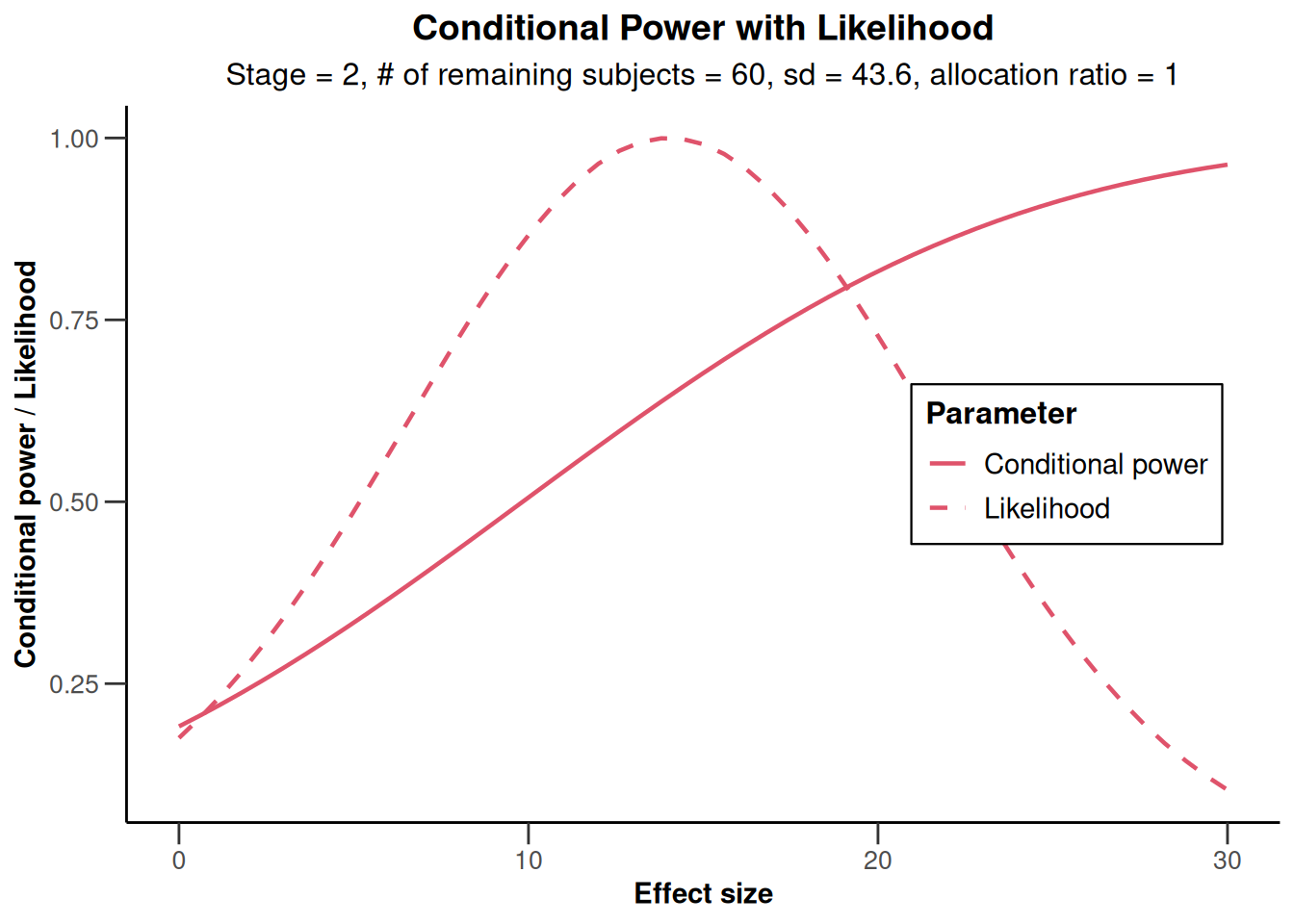
NULLYou can also specify an alternative effect and standard deviation (e.g., thetaH1 = 15, assumedStDev = 35) for which the conditional power should be calculated, and graph the results. Here, the functions getConditionalPower() and getStageResults() are used, but the same result can be obtained when specifying thetaH1 = 15, assumedStDev = 35 in getAnalysisResults().
stageResults <- getStageResults(
  design = designIN,
  dataInput = datasetExample
  )

stageResults |>
  getConditionalPower(
    nPlanned = 60,
    thetaH1 = 15,
    assumedStDev = 35
    )
Conditional power results means
User defined parameters
- Planned sample size: NA, NA, 60
- Assumed effect under alternative: 15
- Assumed standard deviation: 35
Default parameters
- Planned allocation ratio: 1
Output
- Conditional power: NA, NA, 0.7842
stageResults |>
  plot(
    nPlanned = 60,
    thetaRange = c(0, 30),
    assumedStDev = 35
    )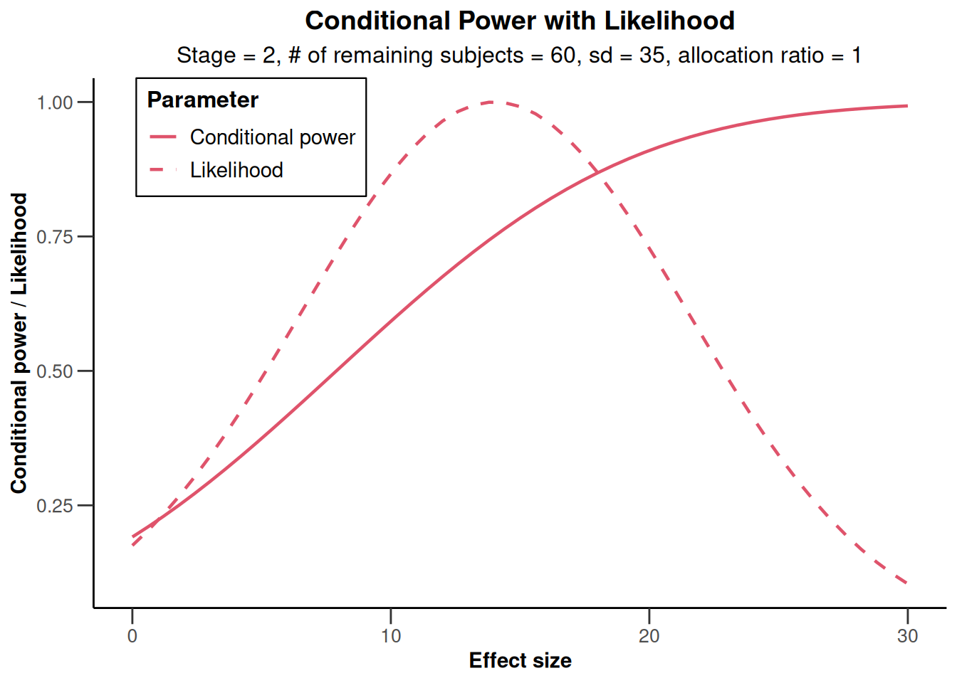
Overall, using a slightly smaller standard deviation than observed, the conditional power calculated with the originally planned sample size seems to be reasonably high.
Final analysis
Assume now that it was decided to continue with the originally planned sample size ( = 60 per stage) and the final stage shows the results:
Final stage:
| arm | n | mean | std |
|---|---|---|---|
| experimental | 32 | 111.3 | 41.4 |
| control | 31 | 100.1 | 39.5 |
We obtain the test results for the final stage and show it as a summary output as follows:
datasetExample <- getDataset(
    means1 = c(112.3, 113.1, 111.3),
    means2 = c(98.1, 99.3, 100.1),
    stDevs1 = c(44.4, 42.9, 41.4),
    stDevs2 = c(46.7, 41.1, 39.5),
    n1 = c(34, 31, 32),
    n2 = c(37, 33, 31)
)

designIN |>
  getAnalysisResults(
    dataInput = datasetExample) |>
  summary()
Calculation of final confidence interval performed for kMax = 3 (for kMax > 2, it is theoretically shown that it is valid only if no sample size change was performed)Analysis results for a continuous endpoint
Sequential analysis with 3 looks (inverse normal combination test design), one-sided overall significance level 2.5%. The results were calculated using a two-sample t-test, equal variances option. H0: mu(1) - mu(2) = 0 against H1: mu(1) - mu(2) > 0.
| Stage | 1 | 2 | 3 |
|---|---|---|---|
| Fixed weight | 0.577 | 0.577 | 0.577 |
| Cumulative alpha spent | 0.0003 | 0.0072 | 0.0250 |
| Stage levels (one-sided) | 0.0003 | 0.0071 | 0.0225 |
| Efficacy boundary (z-value scale) | 3.471 | 2.454 | 2.004 |
| Futility boundary (z-value scale) | -0.500 | 0.500 | |
| Cumulative effect size | 14.200 | 14.016 | 13.120 |
| Cumulative (pooled) standard deviation | 45.614 | 43.604 | 42.432 |
| Stage-wise test statistic | 1.310 | 1.314 | 1.098 |
| Stage-wise p-value | 0.0972 | 0.0968 | 0.1383 |
| Inverse normal combination | 1.298 | 1.837 | 2.128 |
| Test action | continue | continue | reject |
| Conditional rejection probability | 0.0677 | 0.1912 | |
| 95% repeated confidence interval | [-25.271; 53.671] | [-4.803; 32.798] | [0.768; 25.310] |
| Repeated p-value | 0.2978 | 0.0785 | 0.0183 |
| Final p-value | 0.0197 | ||
| Final confidence interval | [0.621; 24.519] | ||
| Median unbiased estimate | 12.620 |
The warning indicates that the calculation of the final CI can be critical if sample size changes were performed. This is not the case here, and so the confidence interval that is based on the stagewise ordering given by (0.621, 24.519) is a valid inference tool. Together with the RCI at stage 3 (0.768, 25.31) it corresponds to the test decision of rejecting the null hypothesis. The test decision is also reflected in both the final \(p\)-value and repeated \(p\)-value being smaller than \(\alpha = 0.025\).
References
- Gernot Wassmer and Werner Brannath, Group Sequential and Confirmatory Adaptive Designs in Clinical Trials, Springer 2016, ISBN 978-3319325606
System: rpact 4.4.0.9305, R version 4.6.0 (2026-04-24), platform: x86_64-pc-linux-gnu
To cite R in publications use:
R Core Team (2026). R: A Language and Environment for Statistical Computing. R Foundation for Statistical Computing, Vienna, Austria. doi:10.32614/R.manuals https://doi.org/10.32614/R.manuals. https://www.R-project.org/.
To cite package ‘rpact’ in publications use:
Wassmer G, Pahlke F (2026). rpact: Confirmatory Adaptive Clinical Trial Design and Analysis. R package version 4.4.0.9305. doi:10.32614/CRAN.package.rpact
Wassmer G, Brannath W (2025). Group Sequential and Confirmatory Adaptive Designs in Clinical Trials, 2nd edition. Springer, Cham, Switzerland. ISBN 978-3-031-89668-2. doi:10.1007/978-3-031-89669-9 https://doi.org/10.1007/978-3-031-89669-9.